Module 7
Caribbean Regional Node

Information | Data | Software | Sites | Feedback | News

This part introduces some of the more advanced features of Bilko for Windows 2.0. Firstly, it looks at the range of file formats supported by the new software. Secondly, the ability to relate image pixels to points on the ground surveyed with Global Positioning Systems (GPS) by means of UTM (Universal Transverse Mercator) coordinates. Thirdly, the making of a colour composite image is briefly explored. Finally, details of how to use Formula documents to manipulate images are given. The last section is primarily for reference purposes.

13. Image file formats

Bilko for DOS (Modules 1-5) and Bilko for Windows 1.0 (Module 6) only supported 8-bit image files. In such images pixels can only take integer values between 0 and 255. This is fine for many purposes and for many satellite sensors data is collected as 6-bit (e.g. Landsat MSS) or 8-bit data (e.g. SPOT XS, Landsat TM) and so can be accommodated. However, other sensors have much higher radiometric resolution. For example, NOAA AVHRR, from which the EIRE2.BMP and EIRE4.BMP images were derived, or the airborne imager CASI (Compact Airborne Spectrographic Imager) collect data as 10-bit (on a scale of 0 to 1023) or 12-bit data (on a scale of 0 to 4095) respectively. To take full advantage of such high radiometric resolution optical data and data from microwave sensors, and to display and store images output after atmospheric correction procedures, Bilko for Windows 2.0 allows images to be stored in three main formats.

• Byte (8-bit integer) - each pixel is stored as a single byte (e.g. .BMP, .GIF files)
• 16-bit integer - each pixel is stored as two bytes (a "word")
• Float (32-bit floating point) - each pixel is stored as four bytes

You will now read in a 16-bit integer file imaged by CASI which has been exported from ERDAS Imagine (a commercial remote sensing package) as a binary flat file (.BIN) extension (CASI2INT.BIN). Each pixel in this image is 1 x 1.1 m in size (so the spatial resolution is 1000x better than the AVHRR images you've been studying). The image is 452 pixels wide and made up of 317 scan lines.

Activity: Use File, Open to start the process of opening CASI2INT.BIN. Bilko for Windows needs more information from you to open this file and so an Open As dialog box appears. There is no header, so leave the Header length (in bytes): entry as 0. Put the correct values (see above) in the Pixels per Line: and Number of Lines: boxes. Now move to the Pixel Format drop-down menu box and select Integer (16 bits). The program now has enough information to open the file, so click on .

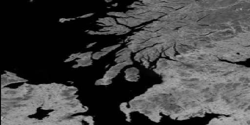
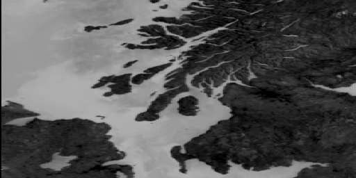
Click on  in the Extract dialog box. Note that a Pixel Values dialog box then appears indicating that the minimum pixel value in the image is 626 and the maximum is 3988 and then click on  again. You will now see the image which shows a seagrass bed off South Caicos Island in the West Indies. See below for a labelled picture to help you orientate yourself. To brighten the image a little, open and apply the pre-prepared stretch CASI2INT.STR.

To display the image on your monitor which displays 256 grey levels, Bilko for Windows has to map the underlying pixel values to a 0-255 scale. It does this automatically when you open the file.

So far you have just used row and column coordinates. Bilko for Windows 2.0 also allows the use of Universal Transverse Mercator (UTM) grid system coordinates which are now widely used for surveys. Most Global Positioning Systems (GPS) allow you to read off where you are on the Earth's surface in UTM coordinates. To classify images (relate pixel values to objects of interest on the ground), field survey is required to collect data on for example, habitat types at a series of known positions on the ground. In this section you will reference the CASI2INT.BIN image to UTM coordinates. You are supplied with a position fix for the top left hand corner of the image which has Easting 237430 and Northing 2378282 for UTM grid zone 19.

Activity: Whilst the CASI2INT.BIN image is the current window, select Edit, Coords to enter the UTM coordinates. This will bring up the Set Coordinates dialog box. Enter the appropriate values (see above) in the Easting (X): and Northing (Y): boxes. The pixel size is 1.0 m wide by 1.1 m along-track. Enter these values in the Pixel Size (metres) boxes for Width (DX): and Length (DY): respectively and then click on .

Now that you have entered the UTM coordinates of the top left of the image (which has been previously geometrically corrected) the Bilko program can calculate the UTM coordinates of any pixel. To use the UTM coordinates rather than row and column coordinates click on View, Coords. Note that the two panels on the Status Bar which did have row and column coordinates now display UTM coordinates. If you click on View, Coords again you can switch back to row and column coordinates. With View, Coords checked use Edit, Go To... function to put the cursor at UTM position 237760, 2378193.

Question 7: Where on the image is the UTM coordinate 237760, 2378193? Answers

Activity: To save the image with its coordinate information, you can save it in Bilko.DAT format. Select File, Save and in the File Save As dialog box, select the file type as Bilko.DAT and click on . Close the file and then re-open it. Note that now Bilko for Windows knows the file size and type and that if you select View, Coords the UTM coordinates become available. Close the file which will not be needed again.

15. Making colour composites

In this section you will briefly explore how to make a colour composite image, in which images taken in three different wavebands are each displayed on a different colour gun on your monitor. Your monitor has Red, Green and Blue (RGB) colour guns each of which can take any intensity value between 0 and 255. When you "connect" three images (using Image, Connect) you can assign them to the different colour guns using the connect toolbar. In this exercise you will take selections of three bands of a Landsat Thematic Mapper (spatial resolution = 30 m) image of Red Sea desert coastline and make them into colour composite images.

For the first colour composite we will put the red waveband (TM3CC.GIF) through the red gun (button 1), the green waveband (TM2CC.GIF) through the green gun (button 2), and the blue waveband (TM1CC.GIF) through the blue gun (button 3). The button numbers correspond to the RGB gun order (R=1, G=2, B=3). Since the Landsat TM wavebands being used roughly correspond to the colours we see, the colour composite should look a bit like how we would see this area from space.
 

Activity: Click on the third button first to make TM3CC.GIF display through the red gun. A red 1 will appear on the button. Then click on the second button to make TM2CC.GIF display through the green gun. A green 2 will appear on the button. Finally, click on the first button to make TM1CC.GIF display through the blue gun. A blue 3 will appear on the button. We are not interested for now in the fourth image so we leave the last button alone. The connect toolbar should now look like this.

16. More on Formula documents

This section assumes that Part 4, section 10 of the Introduction has already been completed. It is essentially a reference for those wishing further to explore Formula documents. Those with some knowledge of computer programming or a good knowledge of using formulas in spreadsheets will find Formula documents fairly straightforward. Those without such a background will probably find them rather daunting! The information here can also be obtained using the Bilko for Windows on-line Help facility.

Each Formula document consists of a series of executable statements, each terminated by a semi-colon `;'. Images are referred to by the @ symbol followed by a number which refers to the connect toolbar buttons and maps to an image in the connected images window. Unless only part of a referenced image has been selected, the Formula document will operate on every pixel in the images so referenced. Images have to be connected and the connect toolbar mapping set up, before they can be operated on by Formula documents.

This section will look at:

Comments make formulae comprehensible both to others and (when you come back to them after some time) to yourself. It is good practice to include copious comments in your formula documents.

Comments are any lines preceded by the hash symbol #.

An example of a set of comments at the start of a formula document is given below:

16.2 Operators

Formula documents support a range of arithmetic, relational (comparison), and logical operators to manipulate images.
 

When several operations occur in a Formula document statement, each part is evaluated in a predetermined order. That order is known as operator precedence. Parentheses can be used to override the order of preference and force some parts of a statement to be evaluated before others. Operations within parentheses are always performed before those outside. Within parentheses, however, normal operator precedence is maintained. When Formula document statements contain operators from more than one category, arithmetic operators are evaluated first, relational operators next, and logical operators are evaluated last. Among the arithmetic operators, exponentiation (^) has preference (is evaluated first) over multiplication/division (*, /), which in turn have preference over addition/subtraction (+, -). When multiplication and division (or addition and subtraction) occur together in a statement, each operation is evaluated as it occurs from left to right (unless parentheses direct otherwise).

Thus the formula statement (@1/91 * -1 + 1) * @2 ; [Part 4, section 10] will divide every pixel in the connected image referenced by @1 (corresponding to button 1 on the connect toolbar) by 91, multiply each pixel of the resultant image by -1 and then add 1 to each pixel in the image resulting. The image referenced by @2 is then multiplied by the result of all these operations.

However, the formula @1/91 * -1 + 1 * @2 ; would start the same way but after multiplying the result of @1/91 by -1 it would then multiply each pixel of image @2 by 1 (having no effect) before adding the output of this operation to the image resulting from @1/91*-1. This is because the second multiplication (1 * @2) takes precedence over the addition before it. The parentheses in the first equation ensure the addition takes place before the second multiplication.

16.3 Functions

The following functions are supported within Formula documents. The argument which you wish the function to act on is enclosed in parentheses). For the trigonometric functions (sin, cos, tan and arctan) the argument is in radians (not degrees).

A few functions which may be a use in remote sensing (e.g. in radiometric correction or bathymetric mapping) and which can be easily derived from these basic functions are listed below.

16.4 Setting up of constants

Constants, like comments, make formulae easier to understand, particularly complex formulae, and can make formulae much easier to alter so that they can be applied to different images. Constant statements should be inserted at the start of formula documents. The form of the statement is:
 

CONST name = value ;

Where the keyword CONST alerts the program processing the formula document to the fact that this is a constant declaration. The name can be any string of alphanumeric characters (but beginning with a letter) which signifies what the constant refers to and the value is an integer or decimal which will be assigned to the name. The constant statement assigns the value to the name so that in formula you can use the name instead of typing in the value. If the constant is something like -1.0986543 and appears lots of times in the formula document, or you wish to experiment with several different values for a constant, having only to change one constant statement can be very useful. Some examples of constant statements are given below.

const Lmin = -0.116 ; const Lmax = 15.996 ;
const pi =3.14152 ;
const dsquared = 1.032829 ;
const cosSZ = 0.84805 ;
const ESUN = 195.7 ;
#
# Converting L to exoatmospheric reflectance (ER) with formulae of the type:
# pi * L * d? / (ESUN * cos(SZ)) ;
@2 = pi * (Lmin + (Lmax/254 - Lmin/255)*@1) * dsquared / (ESUN * cosSZ) ;

In the example above, involving radiometric correction, the values of Lmin, Lmax and ESUN vary for different wavebands. Changing three of the constant values allows the formula to be used for different wavebands with less chance of error. Note also that more than one statement can be typed on one line.

You can also use constant statements to set up labels for images. For example,

This also improves the understandability of formula documents and means you can more easily use formula documents which perform specific functions on a range of images, only having to change the constant statement assignments at the beginning to use with different connected images.

16.5 Conditional statements

To illustrate the use of conditional (IF ... ELSE ...) statements we will look at how they could be used to make a mask from EIRE2.BMP. Sea pixels in EIRE2.BMP have values of 45 or less. Land pixels have values in excess of 45. We will set up this threshold value as a constant called "Threshold". The landmask should have all land pixels set to 0, and all sea pixels set to 1.

The following conditional statement which has one equality comparison (==), one inequality (<), one logical (OR) and two assignment operations (=) within it does the same as the first formula in section 16.2 above (makes a land mask from EIRE2.BMP).
 

CONST Threshold = 45 ;

CONST Eire2 = @1 ;

CONST Landmask = @3 ;

IF ((Eire2 == Threshold) OR (Eire2 < Threshold)) Landmask = 1

ELSE Landmask = 0 ;

The statement says: IF the pixel value in @1 (EIRE2.BMP) is equal to the constant Threshold (45) or is less than the constant Threshold, then assign a value of 1 to the corresponding pixel in @3 (the blank image) ELSE assign a value of 0 to @3. Thus all sea pixels (equal to or below the threshold) are set to 1 and land pixels (above the threshold) are set to zero.

CONST Threshold = 45 ;

CONST Eire2 = @1 ;

IF ((Eire2 == Threshold) OR (Eire2 < Threshold)) 1

ELSE 0 ;

Thus if no image @n is assigned for the output of the Formula document then a new image is created to receive it.

Question 7

At the seaward end of the pier.

Question 8

The formula could be simplified by replacing the long-winded comparison (equal to OR less than) with a single less than or equal to relational operator, thus:
 

CONST Threshold = 45 ;

CONST Eire2 = @1 ;

CONST Landmask = @3 ;

IF (Eire2 <= Threshold) Landmask = 1

ELSE Landmask = 0 ;

The Bilko for Windows software was written by M. Dobson and R.D.Callison. This Introduction was written by A.J. Edwards with help from M. Dobson, J. McArdle, E. Green, I. Robinson, C. Donlon and R.D. Callison and is partly based on the original Bilko tutorial written by D.A. Blackburn and R.D. Callison. HTML release in CW Caribbean by  Joaquin A. Trinanes

Back to main page

Back to Educational Res.

USDOC | NOAA | NESDIS | CoastWatch