Module 7
Caribbean Regional Node

Information | Data | Software | Sites | Feedback | News

You have used the cursor to investigate the pixels making up the image EIRE4.BMP and seen how the brightnesses of sea, land and inland lough (= lake) pixels vary. One feature you should have noted is that land and sea pixels are clearly distinguishable on the basis of brightness values (DNs) in AVHRR band 4. Also the values of land pixels are distinct from Lough Neagh pixels, but the latter overlap in brightness with sea pixels. A good way of seeing whether pixels fall into natural groupings on the basis of their reflectance/emittance in a particular waveband is to study a frequency histogram of brightness values.

4. Histograms

To create a histogram of all the pixel values in an image document you first need to select the whole image file.

 
Activity: Click on the EIRE4.BMP image window to ensure that it is the active window. Click on Edit and then Select All or use the short-cut keys <Shift>+<Spacebar> (or <Ctrl> +A) to select the whole image. Then click on File and New to bring up the dialog box to the right. Since you want to create a Histogram and the HISTOGRAM Document option is already highlighted you can click on  or press <Enter> to generate the histogram.

Note that the histogram is bimodal (has two peaks). From your earlier study of the image using the cursor you will realise that the lower peak (i.e. that covering pixel brightness values with DNs from about 10-70) is composed mainly of land pixels, whilst the upper peak (i.e. that covering pixel brightness values with DNs from about 130-175) is composed mainly of sea pixels.

Click on the histogram and a vertical line will appear. You can use the mouse or the left and right arrow keys to move this line through the histogram. The arrow keys by themselves move the line 10 brightness values at a time to right or left. To move one brightness value at a time hold down the <Ctrl> key and then press the appropriate arrow key. Make sure the Status Bar is in view. In the bottom right hand corner you will see four panels which record firstly, the % of pixels in the image with the brightness value (DN) highlighted; secondly, the start and finish values of the range of DN values highlighted (if only one DN value is highlighted, these will be the same); and lastly the absolute number of pixels in the image with values in the highlighted range. In the example above the upper (sea) peak between DN values of 130 and 180 has been highlighted and the Status Bar shows that there are 50,114 pixels in the image with values of 130-180 and that these account for 38.23% of the EIRE4.BMP image area. Move the cursor-line across the histogram and the display will change accordingly. To select a range of DN values, hold the left mouse button depressed and drag the mouse to right or left.

Minimise the histogram window using the minimize button (Windows 3.1).

Activity: Click on Edit, Selection, Box or click on the box button (left) on the toolbar. Then click near the top left hand corner of the sea in the EIRE4.BMP image and holding down the left mouse button drag the mouse until a rectangular area of sea is outlined with bottom right hand coordinates around pixel (118, 141)å. [Look at Status Bar to see the coordinate you have reached]. Then select File, New and open a new histogram for the pixels inside the box. You will see a histogram with one peak (unimodal) which shows that the sea pixels in the area you have selected range from a DN of about 132-175 in brightness. 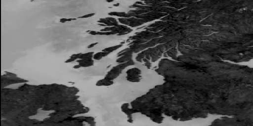Note that the legend above the histogram indicates the top-left and bottom-right pixel coordinates and will look something like the text to the right. Repeat the same exercise with a box of entirely land pixels on the Scottish mainland (see Figure 1). You should get a unimodal histogram with pixel brightness values between 0 and about 70.

åNote: fine positioning of the bottom right hand corner of the box can be achieved using the keyboard. If you need to do this, hold down <Shift>+<Ctrl> and use the arrow keys to extend your selection.

When you have done this, close these last two histogram windows of the sea and land pixels (do not save changes) but leave the histogram of the whole image minimised as you will need this later.

The activities above indicate the kind of information you can find out from studying the histogram (frequency distribution of pixel brightness values) of an image. One of the first things one usually does after loading an image is thus to inspect its histogram to see whether i) all pixels clump together in one peak or whether there are two or more separate peaks which may correspond to different areas of interest on the image, ii) whether pixels are spread over the full range of brightnesses or lumped together causing poor contrast.

The histogram of EIRE4.BMP confirms that the image is not optimally displayed; that is, it is rather dark and it does not utilise the full range of display DNs available and so is somewhat lacking in contrast. To rectify this we can adjust how we display the pixel values by a process known as contrast stretching. As the word stretching implies the process causes the pixels to be displayed over the full range of 256 brightness values (DNs) available.

5. Stretches

The Stretch menu offers seven options:

The picture to the left compares the histogram of the unstretched image (above, left) where the maximum pixel brightness was 178 with that of the image after an automatic linear stretch where the pixel DNs have been spread out over the full range of display brightness values (below, left). Thus those pixels that had a brightness value of 178 now have a value of 255. In mathematical terms the original pixel values have been multiplied by 255/178, this being the simplest way to make use of the full display scale in the present case.

You can check this by examining the pixel brightness values at which the modes in each peak now occur. If you look at the mode in the upper peak (sea pixels) you should find that it now occurs at a pixel brightness value of 219 (=153x255/178). Similarly the lower peak (land pixels) mode has moved from a pixel brightness value of 34 to one of 49 (=34x255/178).

Having stretched the image, you have changed the display values of the pixels which will now be different from the underlying data values.

 
Activity: Click on the  (No selection) button and select Edit, GoTo to put the cursor on (x, y) coordinates 90, 135. Note that now the last panel on the Status Bar shows that this pixel now has a display value of 249 (=174x255/178). The underlying image data values, however, remain unchanged.

Close the histogram of the automatic linear stretched image (without saving it). Then select the EIRE4.BMP image window and use Stretch, Clear to remove the stretch before the next exercise.

 
Activity: Make sure you have selected all of the image file EIRE4.BMP, then from the Stretch menu choose Manual. The graph that appears (right) is the default Look Up Table (LUT) and shows that the pixel brightness values (grey tones) in the image (x-axis) are mapped linearly onto the display scale (y-axis) with no change. Thus an image pixel with value 0 is displayed with brightness 0 whilst one with value 178 is displayed with brightness 178. Stretching involve changing this mapping to take full advantage of the 256 grey levels available on the display. Position the mouse pointer on the stretch graph on the y = x line running from (0, 0) to (255, 255) at around coordinates (175, 175) and double-click on the line. A small flashing box should appear on the line. (If it doesn't, try again). This is called a `knee-point' and can be used to change the mapping of image to display values. As a first try we will mimic the automatic linear stretch you have just performed. This involves increasing the slope of the line so that although pixels with value 0 in the image still map to 0 on the display scale, the maximum image pixel value of 178 maps to 255. To do this the knee-point should be dragged upwards until the Status Bar shows it to be at coordinates (178, 255) and it look like the inset to the right. When you have done this you need to Copy the stretch to the image document. To do this, click on Edit, Copy, or the copy toolbar button ,then click on the unstretched image of EIRE4.BMP and click on Edit, Paste, or the paste toolbar button .

Once you are satisfied that the stretch has altered the histogram as expected, close the histogram window.

From your earlier studies of the image you will have discovered that pixels with brightness values between 0 and about 62 on the EIRE4.BMP image are land. We are not interested in the land and can thus map all these pixel values to 0. The remaining pixels in the image with values from 62-178 represent freshwater lakes (loughs in Ireland and lochs in Scotland) and sea. We can stretch these even more if we make a second knee-point.

Activity: Click on your manual stretch document to make it active again. When you have done this double-click on line above about 60 on the x-axis to make a second knee-point. Drag this one downwards to the x-axis until the Status Bar shows the mapping (62, 0) (it will read 062 000). The stretch should now look like the one shown below.

To copy the stretch to the image, click on Edit, Copy or the copy toolbar button then click on the unstretched image of EIRE4.BMP and click on Edit, Paste or the paste toolbar button .

Note that the land now goes completely black with inland freshwater areas standing out well and the sea showing a lot more detail than the ordinary stretch.

This stretch will be useful later and should be saved:

Activity: Click on your manual stretch document to make it active. Before you save your stretch you should label it so it is clear what it is, so click on the Options menu and select the Names option. This brings up the Names dialog box. This has three boxes to fill in: Chart Name:, X Axis, and Y Axis. You can move between these by clicking in them with the mouse or by using the <TAB> key. In the Chart Name: box, type [without the quotes] "Stretch of sea with land set to 0", in the X Axis box type "Measurement scale DN" as these are the digital numbers actually measured by the satellite sensor^å, and in the Y Axis box type "Display scale DN" as these are the digital numbers which are actually displayed on the screen for pixels with these measured values. When you have done this click on OK.

Now click on the File menu and select Save. In the File, Save As dialog box type EIRE4.STR in the File Name: box and click . Your stretch is now saved for future use. To clear the workspace click on File, Close (or in Windows95 on the window close button) to close the stretch document.

If you are taking a break (recommended!), close EIRE4.BMP.

If you are carrying straight on to the next part, use Stretch, Clear to remove the stretch on EIRE4.BMP.

We could further refine this stretch for oceanic water pixels, if we wished, by inserting a third knee-point and reducing the amount of the display scale used by non-oceanic water pixels with DN values between 62 and about 130. This then allows maximal stretching of image pixels in the sea with values from 130-178.

So far you have displayed the images as a set of grey scales with black representing pixels of DN 0, and white representing pixels of DN 255. However, you can control the display in great detail and assign colours to pixels with certain brightnesses (DN values) to create thematic maps. In the next part of the introduction you will investigate how to do this.
 
 

Question 3

3.1 The DN value of the brightest pixels is 178.

3.2 The maximum which can be displayed is 255. 178 is 69.8% of maximum brightness.

3.3 The modal DN value of the lower (land) peak is 34. There are 3246 pixels with this value in the image.

3.4 The modal DN value of the upper (sea) peak is 153. There are 3668 pixels with this value in the image.

3.5 55.28% of the pixels have values between 0 and 62 and can be classed as land pixels.

3.6 87,766 km? to the nearest square kilometre.

Back to main page

Back to Educational Res.

USDOC | NOAA | NESDIS | CoastWatch