 |
 |
Module 7 |
| Caribbean Regional Node | ||
|
|
Module 7 |
| Caribbean Regional Node | ||
 Part
4
Part
4
Part1 | Part2 | Part3 | Part5
Introduction to the Bilko for
Windows 2.0
image processing software
9. Image menu

The Image menu initially offers two options:
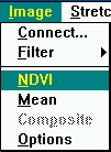
The NDVI (Normalised Difference Vegetation Index) option calculates the NDVI of two images using the following formula (for 8-bit images), where Image 1 is a near infra-red image and Image 2 is an image in the visible red waveband:
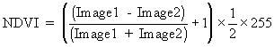
Note: the operation `image 1 - image 2' subtracts the DN of each pixel in image 2 from the DN of the corresponding pixel in image 1.
This option will be dealt with in a specific lesson dealing with images taken in these wavebands. It will not be considered further in this Introduction.
Once two or more images have been `connected' they can have arithmetic performed on them using instructions typed into a Formula Document. These arithmetical manipulations allow specific features of interest in the images to be enhanced or investigated using data from several images at once. These might be images of a given area in one waveband taken at different times, or images in several different wavebands of the same area.
As an exercise to demonstrate how Formula documents work we will create a `mask' using EIRE2.BMP and apply this to EIRE4.BMP to make an image which has all the land with a DN of 0, but has all the sea with the values originally recorded in EIRE4.BMP.
The first step is to create a `mask' from EIRE2.BMP which has all sea pixels with a DN of 1, and all land pixels with a DN of 0. If you explore EIRE2.BMP using the cursor and the zoom facility you will find that almost all sea and lake pixels have a DN of 0 but that some in narrow channels (e.g. in the sound between Islay (Figure 1) and the island of Jura to the east) and close to coasts have DN values up to 45. Land pixels, however, tend to have DN values in excess of 90. To make sure all the sea values are consistently 0 we will firstly divide the image (i.e. will divide the DN of each pixel in the image) by twice 45 plus 1. This ensures that all pixels with values of 45 or less will become 0 (when the result of the division is rounded to the nearest positive integer). Thus 45/91=0.4945 which to the nearest integer is 0, whilst 46/91=0.5055 which to the nearest ineteger is 1. Having done this all sea areas will have a DN of 0 and all land areas will have a DN of 1 or more. If we multiply the image by -1, all land areas will take on negative values but sea areas will remain 0. If we then add 1 to the image, the sea areas will have a DN of 1 whilst the land areas will have DNs of 0 or less which will display as 0 since we can only have DN values between 0 and 255 in an image.
Before we open the Formula document, note that in formulae you refer to images by the @ sign followed by their number on the connect buttons. Thus in this case EIRE2.BMP is image @1 and EIRE4.BMP is image @2.
@1/91*-1+1;
This takes EIRE2.BMP (@1) divides it by 91, multiplies it by -1, and then adds 1 to the resultant image. Note that the formula must finish with a semi-colon (;).
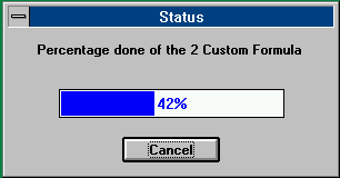
To apply the formula, click on the copy button, then click
on the connected images and click on the paste button. A Status
dialog box will appear which indicates that the formula is being applied.
When the image arithmetic is completed a new image will appear which contains
the results of the manipulation. In this case the image will appear completely
black because pixels have DN values of either 0 or 1. To see the mask clearly,
perform an automatic linear stretch. This maps all the sea pixels with
DN 1 to a display scale DN of 255 so that land appears black and sea appears
white. Use the cursor in conjunction with the Status Bar to check that
the mask's pixel values are either 0 or 1. Your mask should look
like the image below.
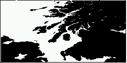
If this mask is applied to another image by multiplying that image by it, it will cause all land pixels to become zero. However, it will not affect sea pixels because it just multiplies them by one. Having looked at the mask image, close it.
The next step is to edit the formula so as to multiply EIRE4.BMP (@2) by the mask. You will now need some parentheses in the formula to make sure the operations are carried out in the correct sequence. Return to you Formula document and edit the formula until it is exactly as below:
(@1/91*-1+1)*@2;
The mask will now be applied to EIRE4.BMP creating an
image whose land pixels actually have a DN of 0, rather than just being
displayed as such. Copy the Formula document, click on the connected images
and paste the formula. The resultant image is similar to EIRE4.BMP but
has all the land black. Use the cursor to verify that land pixels are indeed
all zero in value whilst the sea pixels are unchanged. Close the Formula
document and the new image as they are not required later.
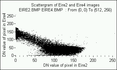
Question 5: Which pixels are in which of the above categories, and why is there this inverse relationship? Answers
Activity: Close the scattergram, the connected pair of images and the EIRE2.BMP image. Do not close EIRE4.BMP as this is needed for the next exercise.
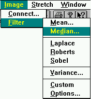
The Filter submenu of
the Image menu allows the user to apply
filtering processes to an image. Six predefined filters (Mean, Median,
Laplace, Roberts, Sobel and Variance) are provided and users are also allowed
to create their own customised filters. The first two predefined filters
act to smooth the image and are sometimes called `low pass'
filters. The middle three act to enhance edges or gradients (i.e.
areas on the image where there are sudden changes in reflectance in a given
waveband) and are sometimes called `high pass' filters. The
predefined Variance filter is a textural
filter which makes areas of changing reflectance appear brighter than relatively
uniform areas which appear darker the more uniform they are.
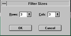
The three predefined high pass filters all act on 3x3
groups of pixels whilst the Mean, Median and
Variance filters can have their sizes
altered in a Filter Sizes dialog box (right).
By default these filters act on 3x3 groups of pixels (3 rows x 3 columns)
and this setting is initially displayed. The maximum size allowed is 15x15
pixels.

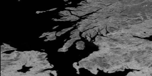
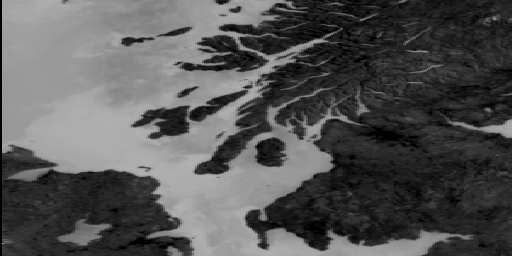
We will now look at the effects of a `high pass', edge enhancing filter. We could use the Laplace, Roberts, or Sobel filters, but will use the Sobel. Details of the different filters is available via on-line Help.
Close the filtered image.
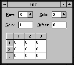
The Image, Filter, Custom
option allows a Custom filter to
be constructed in which the weights (integers) for each cell in the filter
array are defined by the user. We will experiment with constructing a few
3x3 filters to carry out specific modifications to an image. Firstly, we
will construct a simple mean filter for smoothing, and then three different
edge-enhancing, high pass filters. Details of precisely how these convolution
filters work are beyond the scope of this Introduction but are covered
in standard textbooks.
![]()
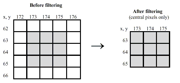
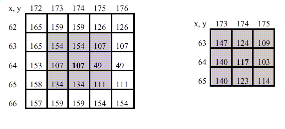
Write the original underlying pixel values (in the second to last panel on the Status Bar) in the 5x5 table below (left). When you are on the correct central pixel, the Status Bar at the right bottom edge of the UNESCO Bilko window should look as follows:
|
|
|
|
|
|
|
|
|
|
|
|
Note the smoothing that has occurred which makes the filtered image look slightly blurred compared to the unfiltered original. Now use the cursor to discover how the central 9 pixels from coordinates (173, 63) to (175, 65) have changed. Enter these values in the 3x3 table above and check that the central pixel is indeed the mean of the nine pixel block of which it is the centre. When you have finished, close the filtered image using its Control box.
Below are three other filters with which to experiment. In each case, edit the Filter document to insert the new cell values, and then copy and paste the new filter to the EIRE4.BMP image. [Note: you can also drag-and-drop filters onto images.]
The second is a filter designed to enhance linear features running in an E-W direction. Examination of EIRE4.BMP indicates that many geological features actually run in a SW-NE direction (e.g. the Great Glen); the third filter is designed to enhance such features.
When you have finished, close all documents and then close
UNESCO Bilko using File,
Exit unless you are continuing on to the advanced options in
Part 5.
Question 5
Pixels with a high DN in EIRE4 but low DN in EIRE2 are sea pixels which absorb near infra-red wavelengths and are thus very dark on EIRE2 but are relatively bright (cool) on the thermal infra-red EIRE4 image. Pixels with a low DN in EIRE4 but high DN in EIRE2 are lowland land pixels which are relatively warm and thus dark in the thermal infra-red EIRE4 image but well vegetated and thus relatively reflective and bright in the near infra-red EIRE2 image. Thus areas which tend to be bright in one image tend to be dark in the other. Highland land areas and lakes provide intermediate values.
Question 6
Coastlines (land/water boundaries) and the oceanic front
north-east of Malin Head.
 |
Back to main page | Back to Educational Res. | USDOC | NOAA | NESDIS | CoastWatch |