 |
 |
Module 7 |
| Caribbean Regional Node | ||
|
|
Module 7 |
| Caribbean Regional Node | ||
Information | Data | Software | Sites | Education | Feedback | News
 Lesson7.
Predicting Seagrass Standing Crop from SPOT XS Satellite Imagery
Lesson7.
Predicting Seagrass Standing Crop from SPOT XS Satellite Imagery
Aim of Lesson
To learn how to derive a map of seagrass standing crop
from a SPOT XS image.
Objectives
2. To investigate the relationship between seagrass standing crop and the single depth-invariant "bottom index" image derived from SPOT XS bands 1 and 2 (green and red wavebands) using field survey data referenced to UTM coordinates.
3. To mask out non-seagrass areas of the SPOT XS depth-invariant image.
4. To construct a palette to display seagrass standing crop densities.
5. To estimate areas of dense, medium and sparse seagrass in the image.
Ecologists and managers of seagrass systems may require a range of data on the status of seagrass habitats. Those parameters which can be measured using remote sensing are listed in Table 7.1.
Table 7.1. Seagrass parameters which can be measured using optical remote sensing. MSS = multispectral scanner, CASI = Compact Airborne Spectrographic Imagery
| Seagrass Parameter | Sensor | Authors |
|
Boundaries of seagrass beds |
Aerial Photography | Greenway and Fry, 1988; Kirkman, 1988; Robblee et al., 1991; Ferguson et al., 1993; Sheppard et al., 1995 |
| Landsat TM | Lennon and Luck, 1990 | |
| Airborne MSS | Savastano et al., 1984 | |
| Seagrass cover (semi-quantitative) | Landsat TM | Luczkovich et al., 1993; Zainal et al., 1993 |
| SPOT XS | Cuq, 1993 | |
| Landsat TM | Armstrong, 1993 | |
| Seagrass biomass/standing crop | CASI, Landsat TM, SPOT XS | Mumby et al., 1997b |
Of the studies listed in Table 7.1, the most detailed obtained a quantitative empirical relationship between seagrass standing crop (biomass of above-ground leaves and shoots) and remotely sensed imagery (Armstrong, 1993; Mumby et al., 1997b). Standing crop is a useful parameter to measure because it responds promptly to environmental disturbance and changes are usually large enough to monitor (Kirkman, 1996). The methods used to map seagrass standing crop are explored in this lesson.
Essentially, this involves five stages:
This lesson relates to material covered in Chapters 12 and 16 of the Remote Sensing Handbook for Tropical Coastal Management and readers are recommended to consult these for further details of the techniques involved. This lesson describes an empirical approach to mapping seagrass standing crop using SPOT XS. The seagrass was located on the Caicos Bank in shallow (<10 m deep) clear water (horizontal Secchi distance 20 - 50 m) and was dominated by the species Syringodium filiforme (Kützing) and Thalassia testudinum (Banks ex König).
The Bilko for Windows image processing software
Familiarity with Bilko for Windows 2.0 is required to carry out this lesson. In particular, you will need experience of using Formula documents to carry out mathematical manipulations of images and Histogram documents to calculate the area of particular features on the imagery. A familiarity with Excel is also desirable.
Image data
This lesson will use a SPOT XS image of the Caicos Bank as this imagery covers a large area while having a reasonably high spatial resolution (20 m). To obtain a quantitative relationship between image data and seagrass standing crop, it is important to compensate for the effects of variable depth. Therefore, the image you are provided with has undergone the depth-invariant processing described in Lesson 5 of this module. SPOT XS bands 1 (green ) and 2 (red) were processed to form a single depth-invariant bottom index band and you are provided with a subset of the Caicos Bank showing South Caicos (file XS_DI.DAT). This is a floating point file where each pixel value is represented by a real number stored in four bytes. To illustrate the importance of compensating for variable depth, when seagrass standing crop was regressed on reflectance (not corrected for depth), the coefficient of variation (r2) ranged from 0.05 - 0.32 for SPOT XS (and was similarly low for other sensors). These values are too low for adequate prediction of seagrass standing crop.
You are also provided with two mask files. The first is a land mask (LANDMSK7.GIF) in which all land pixels are set to zero and all submerged pixels are set to a value of 1. When another image is multiplied by the land mask, all land pixels are set to zero whilst submerged pixels are unaffected. The second mask removes all non-seagrass habitats in the imagery (SEAGMASK.GIF). This was created from an image of coral reef, algal, sand and seagrass habitats (see Lesson 6 for a similar example). Land, coral reef, sand and algal pixels were set to zero leaving only seagrass habitats set to a value of 1.
Field survey data
A variety of techniques exist for measuring seagrass standing crop including destructive and non-destructive approaches. We recommend non-destructive methods because they allow repeated monitoring, are less harmful to the environment and are generally faster than destructive methods. Good general texts on seagrass sampling include Unesco (1990), English et al. (1994) and Kirkman (1996). The non-destructive visual assessment method of Mellors (1991) for estimating seagrass standing crop in situ was modified for use here.
Standing crop is measured in units of dry weight organic
matter per unit area (g. m-2) and is correlated with shoot density
and leaf area index. The visual assessment method uses a linear scale of
biomass categories which are assigned to seagrass samples in 0.25m2
quadrats. A six point integer reference scale of quadrats is used (1-6).
The technique is summarised in Figure 7.1 and a thorough analysis of its
errors and limitations is given by Mumby et al. (1997a).
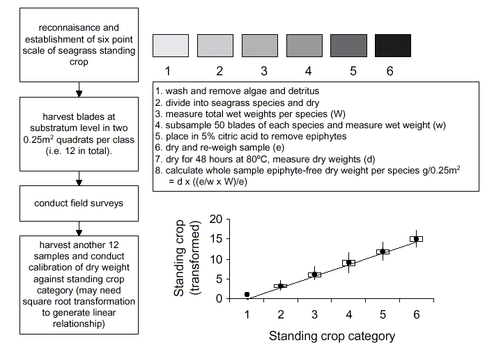
Figure 7.1. Visual assessment of seagrass standing crop
At least 30 seagrass sites should be surveyed and these should represent the entire range of standing crop in the area of interest. The size of each site will depend on the spatial resolution of the remotely-sensed imagery; larger sites are required to represent the standing crop in larger pixels. As a general guideline, we found a 10 m diameter site size to be acceptable for SPOT XS imagery. At each site, the mean standing crop of seagrass is estimated from a number of randomly-placed replicate quadrats. For medium to dense seagrass beds, a sample size of 6 quadrats is probably acceptable. However, a larger sample size should be used in patchier seagrass areas (for further discussion see Downing and Anderson, 1985).
Lesson Outline
This lesson assumes that stage 1, the collection of field data, has already been undertaken using the guidelines set out above. The first practical activity will be the second stage of preparing a map of seagrass standing crop, namely, relating field data to image data to derive a calibration graph.
Relating field data to image data: calibration of SPOT XS data into units of seagrass standing crop (g.m-2)
Although we surveyed the standing crop of 110 seagrass sites, you are provided with the UTM coordinates for five sites (Table 7.2) and the standing crops estimated at these locations during the field survey. Click the no selection button and use the Edit, GoTo command to find the pixel value at each coordinate. Note that the status bar will display the top-left coordinates of the pixel that overlaps the GPS position. Enter the pixel values into Table 7.2 to 4 decimal places. These five points can be used to generate a regression of seagrass standing crop on image data (SPOT XS depth-invariant data). Launch Microsoft Excel and open the workbook file LESSON7.XLS. This file contains three sheets: a data matrix called Lesson, a data matrix called area calculation and a calibration graph. Click on Lesson if this is not the default sheet and enter your values into the table (the table is identical to Table 7.2, except that the coordinates are those of the top-left of the pixels containing the GPS coordinates you enter; i.e. those displayed on the status bar).
|
|
|
|
|
|
|
|
|
|
3.79
|
|
|
|
|
|
200.59
|
|
|
|
|
|
109.20
|
|
|
|
|
|
37.21
|
|
|
|
|
|
57.00
|
Question: 7.1. What is the calibration equation and what do the axes y and x represent?
7.2. What is the coefficient
of determination (r2)?
The calibration equation calculated above was based on only five samples of field data. When we used 110 seagrass sites, we obtained the following equation which is not dissimilar to that which you have already calculated.
y = 38.6 - 5.6x
This is the standard equation of a straight line where 38.6 is the intercept of the line with the y-axis (i.e. the value of y when x = 0), 5.6 is the magnitude of the gradient and the minus sign indicates that the slope is negative (i.e. as x gets bigger, y gets smaller). As the y-axis variable was the square root of seagrass standing crop, the left hand side of the equation must be squared to give values in original units of seagrass standing crop (g.m-2).This can be re-written in a slightly easier format to give:
Seagrass standing crop = [38.6 - (5.6 * depth-invariant SPOT data)]2
The calibration will be implemented at the same time as applying the land mask. Fortunately, seagrass standing crop does not exceed 255 g. m-2 at the study site and therefore, it can be represented directly on an 8-bit image with 256 possible values for each pixel (if this was not the case, standing crop would have to be scaled to 255 values).
Make sure that the Apply stretches to charts, clipboard etc. checkbox is unchecked in the Stretch, Options dialog box. Then select all pixels in the new image, STEP2.GIF and apply a histogram equalization contrast stretch. The seagrass beds will be clearly distinguishable from the land and non-seagrass habitats. Verify the designation of pixel values by clicking on land areas and non-seagrass marine areas - are the pixel values 0 and 255 respectively?
The land and non-seagrass marine pixels will swamp any histogram of the whole image so to see the spread of standing crop values in a seagrass bed you will need to select a subset of pixels. Use Edit, GoTo to select a box or block of pixels in the large seagrass bed near the north-east of the image starting at column and row coordinates 338, 143 with a DX: of 41 and DY: of 36. Use File, New to bring up a HISTOGRAM document of this pixel block.
Question: 7.3. What is the lowest value of the seagrass pixels and what does this represent in terms of standing crop?
7.4. What is the highest standing crop in the block and how many pixels have this standing crop?
7.5. What is the modal standing crop in the seagrass bed (based on this block sample)?
Close the histogram document.
The next step is to create a colour palette to display the seagrass standing crop as five colour-coded categories corresponding to the top five classes on the visual assessment scale. The palette applies to the display image values (mapped by the Look Up Table - LUT) as opposed to the underlying data values. We want to map the underlying data values to colours and so must make sure there are no stretches in operation. Thus before proceeding further we should clear any stretches of STEP2.GIF.
[Hint: Click the upper of the palette boxes beneath the colour space and then set the Red:, Green: and Blue: guns to 127, then repeat for the lower of the two palette boxes, and click on Update. This should set the first cell to grey. To check whether this has worked, copy the palette and paste it to the unstretched STEP2.GIF image. All land areas should become mid-grey].
Next, select the last cell which represents a pixel value of 255 (non-seagrass marine habitats). Set this to cyan (R=0, G=255, B=255) using the same procedure. You must now choose a colour scheme for seagrass standing crop (i.e. the remaining pixels). You can experiment, creating your own scheme and applying your palettes to the image.
For guidance, two palettes have been prepared already (these have land set to black, non-seagrass marine areas to white and seagrass to shades of green. Open the palette document SEAGRAS1.PAL, making sure, as you do so, that the Apply check-box in the File Open dialog box is not checked. This palette was created by selecting all seagrass boxes [Hint: select the first box on your palette, and then select the last while depressing <Shift>] and assigning a pale green colour to the upper palette box and a dark green colour to the lower palette box. Try this on your palette.
When you are ready, close the palette images and STEP2.GIF.
Now that you have created a map of seagrass standing crop, the final objective is to calculate the area of seagrass in each standing crop category. In a practical situation, this might be repeated every few years to monitor changes in the coverage of particular types of seagrass bed.
The total size of the image is 444 x 884 pixels (see top of histogram) so there are a total of 392496 pixels in the image. Place the mouse pointer at any point on the x-axis and view the status bar at the bottom right-hand corner of the display. You will see four sets of numbers. The two middle numbers indicate the lowest and highest values in the range of pixel values which have been highlighted. If only one value has been selected (e.g. by clicking on a particular value on the x-axis) then both values will be the same. The right display is the number of pixels highlighted on the histogram and the left display is the percent of pixels which have been highlighted. This percentage is calculated by dividing by the total number of pixels in the image. Therefore, 10% would equal 10/100 * 392496 pixels (39250 to the nearest whole number).
Use the histogram to determine the percentage of pixels and number of pixels in each standing crop class. For example, the first class represented standing crop from 1 - 5 g.m-2, is displayed as pixel numbers 1 - 5. To estimate the percent of pixels in this class, position the mouse pointer on a pixel value of 1 and drag it to the right until it reaches 5. The percent shown at the bottom of the screen will represent the total percent of pixels in this class (to the nearest 0.01%) and the right hand number will show the total number of pixels that this represents.
Enter both values into the appropriate columns of Table 7.3 and calculate the area of each class in hectares using a calculator. Alternatively, launch Microsoft Excel, open the file LESSON7.XLS and select the sheet "area calculation". This sheet contains Table 7.3 and formulae to automate the area calculation. You can check your working by typing your percent values and numbers of pixels into this table and comparing the area estimates to those calculated by hand. What are the areas of each seagrass class in hectares?
| Seagrass standing crop | Pixel Range |
|
|
|
|
| 1 to 5 | 1 - 5 | ||||
| 6 to 20 | 6 - 20 | ||||
| 21 to 70 | 21 - 70 | ||||
| 71 to 130 | 71 - 130 | ||||
| 131 to 200 | 131 - 200 | ||||
| 201 to 254 | 201 - 254 | ||||
| (units = g.m-2) | |||||
| Land | 0 |
50.47
|
|
|
|
| Non-seagrass | 255 |
40.45
|
|
|
|
Close all files.
A map of seagrass standing crop could be used in several ways. The simplest of these would be the provision of extra information on the status of seagrass beds in a particular area of interest. However, the maps might also be used to identify the location and extent of important fisheries habitats. For example, the juvenile conch (Strombus gigas) is often associated with seagrass habitats of low standing crop (Appeldoorn and Rolke, 1996). Monitoring of seagrass standing crop over time would also be possible, particularly if the remotely sensed data had a high spatial resolution. Changes in standing crop would be displayed in 2-dimensions and possibly related to the causes of the change (e.g. point sources of pollutants). However, if monitoring is going to be undertaken, it is important to quantify errors and assess the confidence with which remote sensing predicts seagrass standing crop. For further details of these methods, readers are referred to Mumby et al. (1997b). Alternatively, a simpler monitoring programme could compare the coverage of seagrass classes from, say, year to year (as outlined in this lesson).
References
Appeldoorn, R.S., and Rolke, W., 1996, Stock abundance and potential yield of the Queen Conch resource in Belize. Unpublished report of the CARICOM Fisheries Resource Assessment and Management Program (CFRAMP) and Belize Department of Fisheries, Belize City, Belize.
Armstrong, R.A., 1993, Remote sensing of submerged vegetation canopies for biomass estimation. International Journal of Remote Sensing 14: 10-16.
Cuq, F., 1993, Remote sensing of sea and surface features in the area of Golfe d'Arguin, Mauritania. Hydrobiologia 258: 33-40.
Downing, J.A, and Anderson, M.R., 1985, Estimating the standing biomass of aquatic macrophytes. Canadian Journal of Fisheries and Aquatic Science 42: 1860-1869.
English, S., Wilkinson, C., and Baker, V., 1997, Survey Manual for Tropical Marine Resources, 2nd Edition. (Townsville: Australian Institute of Marine Science).
Ferguson, R. L., Wood, L.L., and Graham, D.B., 1993, Monitoring spatial change in seagrass habitat with aerial photography. Photogrammetric Engineering and Remote Sensing 59: 1033-1038.
Greenway, M., and Fry, W., 1988, Remote sensing techniques for seagrass mapping. Proceedings of the Symposium on Remote Sensing in the Coastal Zone, Gold Coast, Queensland, (Brisbane: Department of Geographic Information) pp. VA.1.1-VA.1.12.
Kirkman, H., 1996, Baseline and monitoring methods for seagrass meadows. Journal of Environmental Management 47: 191-201.
Kirkman, H., Olive, L., and Digby, B., 1988, Mapping of underwater seagrass meadows. Proceedings of the Symposium Remote Sensing Coastal Zone, Gold Coast, Queensland. (Brisbane: Department of Geographic Information) pp. VA.2.2-2.9.
Lennon, P., and Luck, P., 1990, Seagrass mapping using Landsat TM data: a case study in Southern Queensland. Asian-Pacific Remote Sensing Journal 2: 1-6.
Luczkovich, J.J., Wagner, T.W., Michalek, J.L., and Stoffle, R.W., 1993, Discrimination of coral reefs, seagrass meadows, and sand bottom types from space: a Dominican Republic case study. Photogrammetric Engineering & Remote Sensing 59: 385-389.
Mellors, J.E., 1991, An evaluation of a rapid visual technique for estimating seagrass biomass. Aquatic Botany 42: 67-73.
Mumby, P.J., Edwards, A.J., Green, E.P., Anderson, C.W., Ellis, A.C., and Clark, C.D., 1997a, A visual assessment technique for estimating seagrass standing crop. Aquatic Conservation: Marine and Freshwater Ecosystems 7: 239-251.
Mumby, P.J., Green, E.P., Edwards, A.J., and Clark, C.D., 1997b, Measurement of seagrass standing crop using satellite and airborne digital remote sensing. Marine Ecology Progress Series 159: 51-60.
Robblee, M.B., Barber, T.R., Carlson, P.R., Jr, Durako, M.J., Fourqurean, J.W., Muehlstein, L.K., Porter, D., Yarbro, L.A., Zieman, R.T., and Zieman, J.C., 1991, Mass mortality of the tropical seagrass Thalassia testudinum in Florida Bay (USA). Marine Ecology Progress Series 71: 297-299.
Savastano, K.J., Faller, K.H., and Iverson, R.L., 1984, Estimating vegetation coverage in St. Joseph Bay, Florida with an airborne multispectral scanner. Photogrammetric Engineering and Remote Sensing 50: 1159-1170.
Sheppard, C.R.C., Matheson, K., Bythell, J.C. Murphy, P., Blair Myers, C., and Blake, B., 1995, Habitat mapping in the Caribbean for management and conservation: use and assessment of aerial photography. Aquatic Conservation: Marine and Freshwater Ecosystems 5: 277-298.
Unesco, 1990, Seagrass Research Methods. Monographs on Oceanographic Methodology, 9. (Paris: Unesco).
Zainal, A.J.M., Dalby, D.H., and Robinson, I.S., 1993, Monitoring marine ecological changes on the east coast of Bahrain with Landsat TM. Photogrammetric Engineering & Remote Sensing 59: 415-421.
Answers to Questions
Table 7.2. Relating image data to field-measured estimates of seagrass standing crop at a series of GPS coordinates.
|
|
|
|
|
|
|
|
|
|
|
3.79
|
|
|
|
|
|
200.59
|
|
|
|
|
|
109.20
|
|
|
|
|
|
37.21
|
|
|
|
|
|
57.00
|
In the block of 41 x 36 seagrass pixels starting at
coordinates 338, 143:
| Seagrass standing crop | Pixel Range |
|
|
|
|
| 1 to 5 | 1 - 5 |
1.70
|
|
3530546
|
353.1
|
| 6 to 20 | 6 - 20 |
3.44
|
|
7144674
|
714.5
|
| 21 to 70 | 21 - 70 |
2.11
|
|
4375359
|
437.5
|
| 71 to 130 | 71 - 130 |
1.39
|
|
2889927
|
289.0
|
| 131 to 200 | 131 - 200 |
0.40
|
|
828943
|
82.9
|
| 201 to 254 | 201 - 254 |
0.03
|
|
71944
|
7.2
|
| Land | 0 |
50.47
|
|
104795429
|
10479.5
|
| Non-seagrass | 255 |
40.45
|
|
83993562
|
8399.4
|
 |
Back to main page | Back to Module 7 | USDOC | NOAA | NESDIS | CoastWatch |