CoastWatch Caribbean Regional Node: Bilko Lessons

		Module 7
Caribbean Regional Node

United Nations Educational, Scientific and Cultural Organization

Lesson 1. Visual Interpretation of Images with the Help of
Colour Composites: Getting to Know the Study Area

Aim of Lesson

To learn how to interpret satellite and airborne digital imagery visually, relate features revealed on images to features on the Earth's surface, and use images to help in planning field survey.

Objectives

1. To become proficient in preparing colour composite images.

2. To use field reconnaissance data to assist in visually interpreting images.

3. To see how satellite and aerial imagery may be used to aid planning of field surveys.

Overview of Lesson

A simple visual interpretation of remotely-sensed imagery can often reveal considerable detail on the nature and distribution of habitats in the area of interest. Visual interpretation is the identification of features based on their colour, tone, texture and context within the imagery. To visually interpret digital data such as satellite images, individual spectral bands must be displayed simultaneously in the form of a colour composite. For example, Landsat TM bands 1, 2 and 3 (Appendix 1.1) broadly represent the blue, green and red parts of the electromagnetic spectrum (ES). When these bands are fed through the corresponding blue, green and red "colour guns" of a computer monitor, the resulting image strongly resembles what our eyes would see from the sensor's vantage point. We thus have an intuitive understanding of the colours presented and can usually make an informed interpretation of the scene (e.g. dark blue probably represents deep water). Such images are called true colour composites (TCC).

This lesson begins by describing how to make a colour composite image from the spectral bands of SPOT XS (Appendix 1.2). SPOT XS does not have a spectral band in the blue component of the ES, so the composite is biased towards longer (red) wavelengths and is known as a false colour composite (FCC). However, false colours can still be related to habitats of interest and photographs are provided to relate the FCC to some of the mangrove habitats present in the area represented by the image. The other marine habitats described throughout this module are then introduced by visually interpreting an image of Cockburn Harbour, South Caicos which was acquired using an airborne multispectral digital sensor called the Compact Airborne Spectrographic Imager (CASI: see Appendix 1.3).

Field work is an essential part of any remote sensing study and the lesson ends with a discussion of how visual interpretation can aid the planning of field surveys.

Background Information

Chapters 4 and 10 of the Remote Sensing Handbook for Tropical Coastal Management discuss the use of visual interpretation for planning field surveys and habitat mapping respectively, and readers are recommended to consult this book for further details.

The Bilko for Windows image processing software

Familiarity with Bilko for Windows 2.0 is required to carry out this lesson. Most of the lesson is confined to locating coordinates on images, interpreting images visually and matching areas of habitat on images to photographs taken during field survey.

Image data

All images used in this module are of the Turks and Caicos Islands, to the south-east of the Bahamas. The first image was acquired by a multispectral sensor (XS) mounted on the French SPOT satellites. It was acquired on the 27^th March 1995 at 15:28 hours Universal Time (i.e. at approximately 10:30 local time in the Turks and Caicos). The full extent of this SPOT image is presented in Figure 1.1 but a subset of South Caicos is provided here (see Figure 1.2 for location). SPOT XS has three spectral bands which are represented by the files XS1SUB.GIF (green), XS2SUB.GIF (red), and XS3SUB.GIF (infrared). Each pixel on this image covers 23 x 23 m on the ground/sea.

The second image (CASIHARB.GIF) is a true colour composite of CASI data acquired for Cockburn Harbour (see inset of Figure 1.2). The CASI was mounted on a locally-owned Cessna 172N aircraft using a specially designed door with mounting brackets and streamlined cowling. An incident light sensor (ILS) was fixed to the fuselage so that simultaneous measurements of irradiance could be made. A Differential Global Positioning System (DGPS) was mounted to provide a record of the aircraft's flight path. Data were collected at a spatial resolution of 1 m² in 8 wavebands (Table 1.1) during flights over the Cockburn Harbour area of South Caicos, Turks and Caicos Islands (21^o 30' N, 71^o 30' W) in July 1995. Further details are given in Clark et al. (1997).

Table 1.1. Band settings used on the CASI.

Band	Part of electromagnetic spectrum	Wavelength (nm)
1	Blue	402.5 - 421.8
2	Blue	453.4 - 469.2
3	Green	531.1 - 543.5
4	Green	571.9 - 584.3
5	Red	630.7 - 643.2
6	Red	666.5 - 673.7
7	Near Infrared	736.6 - 752.8
8	Near Infrared	776.3 - 785.4

The CASI image displayed here was acquired at approximately 10 a.m. local time on 16 July 1995. For the purposes of this lesson, a colour composite image has been created already; the resultant file CASIHARB.GIF comprises bands 1, 3 and 5 (Table 1.1).

Figure 1.1. Location of the Landsat and SPOT scenes from which subscenes were taken and areas of two of the larger Landsat subscenes. Showing position on part of Admiralty Chart 1266 of the south-eastern Bahama Islands.

Location Landsat and Spot Scenes

Approximate area covered by whole Landsat TM and MSS scenes (roughly 185 x 185 km) from which subscenes were taken.
Area covered by whole SPOT XS and Pan scenes (60 x 60 km) from which subscenes (see Figure 1.2) were taken. Note that one Landsat scene contains about 9 SPOT scenes.
Approximate area covered by Landsat MSS subscenes used in Lesson 2 (MSS1.GIF-MSS3.GIF) and Landsat TM subscene used in Lesson 4 on mapping bathymetry (TMBATHY1.GIF-TMBATHY4.GIF).
Location of Landsat TM subscenes used in Lesson 3 on radiometric correction.

Figure 1.2. South Caicos area to show locations of principal images used.
Mangrove areas on the west coast of South Caicos are stippled.

Locations of principal images

Boundaries of SPOT XS subscenes used in Lesson 1 and Lesson 2 (XS1SUB.GIF-XS3SUB.GIF).
Boundaries of SPOT Pan subscene used in Lesson 2 (XPSUBSET.GIF).
Location of aerial photographic subscene AP_EAST1.GIF used in Lesson 2.
Location of aerial photographic subscene AP_SCAIC.GIF used in Lesson 2.
Location of CASI (Compact Airborne Spectrographic Imager) images used in Lessons 1 and 2 (CASIHARB.GIF) and in Lesson 5 on water column correction (CASI2C16.DAT-CASI5C16.DAT).
Approximate location of the uncorrected CASI image of mangroves used in Lesson 2 (CASIMANG.GIF).
Location of aerial photographic subscene AP_MANG.GIF used in Lesson 2.
Location of CASI images used in Lesson 8 on assessing mangrove leaf area index (CASIMNG6.DAT-CASIMNG7.DAT).

Lesson Outline

Creation of a false colour composite from SPOT XS data

Activity: Launch Bilko for Windows and open the three band geometrically corrected SPOT XS image. In the File, Open dialog box deselect Extract (if it is checked on). Then select XS1SUB.GIF with the mouse pointer and with the <Ctrl> key held down select XS2SUB.GIF and iXS3SUB.GIF also, then click on OK. This should open all three SPOT XS files at once.

Question: 1.1.How many kilometres wide and long is the SPOT subscene image? Answers

Connect the three images using the Image, Connect function (highlight each with the cursor whilst depressing the <Ctrl> key). Set the connect toolbar so that the third connected image (XS3SUB.GIF - XS near-infra-red band) is 1, XS2SUB.GIF (XS red band) is 2, and XS1SUB.GIF (XS green band) is 3. Then select the Image, Composite function to make a false colour composite. (Remember, the first image clicked is displayed on the red gun, the second with the green gun, and the third with the blue gun - hence, RGB). Select the whole of the colour composite image using Edit, Select All or <Ctrl>+A and experiment with different stretches (AutoLinear, Equalize and Gaussian) to display the colour composite to full advantage. Choose the stretch which gives the greatest visual contrast. [We found the automatic linear stretch to be best]. Keep the colour composite image in the viewer but select and close all other images individually. Do not save any changes to image files.

Question: 1.2. What principal colour is the land in the colour composite? Why is this? Answers

1.3. Between which approximate column and row (x, y) coordinates does the runway on

Visual interpretation of SPOT XS Imagery of South Caicos

Part 1: Identification of mangrove habitats of South Caicos

You are now going to follow a transect across the mangrove fringing the coast starting at the waters edge. Mangrove forests often exhibit well-defined patterns of species zonation from the waters edge to the higher and drier land further within the forest.

Activity: Use the Edit, GoTo command to place the cursor to x, y coordinates 179, 475. If you cannot see the winking cursor, scroll down the image. Position the mouse pointer over the cross and double-click. The image will zoom in. Double-click again. (Note: you can zoom out by depressing <Ctrl> whilst double-clicking). You should note a bright-red (high infra-red reflectance) belt along the west coast of the island which corresponds to a mangrove stand. A northward-facing colour aerial photograph was taken at the position of the cursor. To view the photograph, use File, Open and select MANG_AIR.GIF. The dark green band of mangrove is clearly visible along the waters edge. Close the aerial photograph file.

Click on the false colour composite image and use the Edit, GoTo command to place the cursor at each of the positions in Table 1.2. At each position, open the corresponding photograph which was taken during field work (Hint: Close each photograph before moving on to the next).

Table 1.2. Visual interpretation of SPOT XS data to examine mangrove zonation

Coordinates		Photograph	Notes
X:	Y:	file name
184	472	mang_rms.gif	Fringing stand of short red mangrove (Rhizophora mangle) which is usually found near the waters edge. The mangrove stand continually encroaches seaward making this a dynamic area of mangrove proliferation.
188	472	mang_rmt.gif	A forest of tall R. mangle which can reach 7 m in height.
190	472	mang_bla.gif	An area of tall black mangrove (Avicennia germanians) which is usually found set back from the waters edge in drier environments.
194	472	mang_wht.gif	The short, scrubby white mangrove (Laguncularia racemosa) which is found on higher ground where it is often interspersed with non-mangrove vegetation.

Part 2: Identification of some marine habitats in Cockburn Harbour

The second part of this section will focus on the main submerged habitats of Cockburn Harbour which lies to the south-east of the area you have just viewed for mangrove habitats (see Figure 1.2).

Activity: Use the Edit, GoTo command to place the cursor at coordinates 205, 510. A colour aerial photograph was taken in a south-eastward direction at this point. To view the photograph, use File, Opento select the file COCKHARB.GIF. The coast of Cockburn Harbour is visible and the long island opposite is Long Cay whose northern-most point lies at position 222, 578 in the SPOT image. The foreground of the photograph shows a mosaic of seagrass beds and sand patches. Close the aerial photographic view.

Using the Edit, GoTo command, move the cursor to position 215, 536 in the SPOT composite image. Position the mouse pointer over the cursor and double-click on the image to zoom in further. The image looks very dark in this area because the habitat there is dense seagrass which has a generally low albedo. To see how this seagrass looks underwater, open the file SEAG_DEN.GIF.

Close the photograph and move the cursor a few pixels east to coordinate 218, 537. The reflectance is greater at this position due to the presence of bare sand (you may need to zoom in to a 7:1 ratio to see the brighter pixels). The sand habitat is illustrated in file CCC_SND.GIF.

Once you have completed this part of the lesson, close all files without saving their contents.

Visual interpretation of CASI imagery of Cockburn Harbour Activity: Use File, Open to view the file CASIHARB.GIF which is a pre-stretched false colour composite of Cockburn Harbour taken with the CASI. The wiggly edge to the image is caused by the rolling of the aircraft as it flies along. The image represents the far (eastern) side of Cockburn Harbour as viewed in the aerial photograph, COCKHARB.GIF. The CASI sensor itself can be viewed by opening the file CASI_SEN.GIF showing the instrument mounted in a specially-designed door (for further details see Image data section above and Clark et al., 1997).

Many reef habitats can be identified in this image. To familiarise you with these habitats and describe the skills of visual interpretation, you are provided with a series of column and row coordinates, photographs and interpretation notes (Table 1.3). Use the Edit, GoTo command to relate the location (coordinate) of each site to the habitat. The notes should outline the mental decisions taken when identifying each habitat. Close each photograph before moving on to the next and zoom in and out of the CASI colour composite as necessary (double-click and <Ctrl>+double-click on the image, respectively).

Table 1.3. Visual interpretation of CASI imagery to identify key marine habitats.

Coordinates			Habitat photograph	Description of habitat	Notes on visual interpretation / recognition of habitat on CASI image
X:	Y:	file name
375	118	brown_al.gif		brown algae (Lobophora variegata) dominated	brown colour, often located on hard substrata near the shoreline
351	243	mont_col.gif		large coral heads (Montastraea annularis)	distinctive texture: large dark patches surrounded by paler sand or seagrass
334	366	ccc_palm.gif		large stands of elkorn coral (Acropora palmata)	usually located in shallow areas with high wave energy (e.g. reef crest, seaward side of islands)
222	553	mont_svy.gif		Montastraea reef - a mixed community of corals, algae and sponges. Of the hard corals, the genus Montastraea dominates	associated with the outer fringing reef (seaward of the reef crest or lagoon) and at depths where the wave exposure is reduced (i.e. 5 m plus)
231	513	ccc_snd.gif		sand gully in deep water	high reflectance yet deep water indicating a strongly-reflecting substratum
188	249	gorgplan.gif		plain dominated by soft corals (gorgonian plain)	this habitat often has a high percent cover of bare substratum with a high reflectance. Therefore, its colour lies somewhere between sand and the shallowest areas of Montastraea reef
237	112	seag_den.gif		dense seagrass (Thalassia testudinum)	usually has a distinctive green colour but may appear black in deeper water. Most obvious features are homogenous consistency (texture) and sharp boundaries
289	196	seag_spr.gif		sparse (patchy) seagrass	green in colour but the tone is more luminescent than dense seagrass. Other features are patchy texture and indistinct boundaries
256	146	blowout.gif		seagrass "blowout"	not a habitat but an important feature created by a loss of seagrass within a seagrass bed. Characteristic elliptical shape with high contrast between sand and dense seagrass

Activity: When you have finished studying the photographs and honing your visual identification skills, answer the following questions, giving your reasoning.

Question: 1.4. What habitat would you expect to find at column and row coordinates 220, 52? Answers

1.5. What habitat would you expect to find at coordinates 270, 226?

1.6. What habitat would you expect to find at coordinates 370, 270?

1.7. What habitat would you expect to find at coordinates 80, 440?

1.8. What habitat would you expect to find at coordinates 279, 117?

When you have answered the questions close the CASI colour composite image and think about how you might a) define habitats so that other people will know what you mean, and b) how you might use remote sensing to help plan field surveys.

The habitats you have looked at in this lesson were defined from ecological field data. Bear in mind, however, that one person's understanding of a "habitat type" may vary from the next person's and thus, it is important to make a clear definition of habitats prior to undertaking a study. The objectives of most habitat mapping exercises fall into four groups: (i) ad-hoc definition of habitats without field data,

(ii) application-specific studies focused on only a few habitats,

(iii) geomorphological studies, and

(iv) ecological studies.

An ad-hoc approach to defining habitats is relatively cheap but is only recommended in the cases where the accuracy of habitat maps is not important. Habitat-specific studies (e.g. a seagrass study) should include the habitat of interest and those additional habitats which are most likely to be confused with it (e.g. macroalgae is easily confused with seagrass), thus permitting the accuracy of mapping to be evaluated. Geomorphological classifications can be assigned to imagery with little or no field work. The establishment of objective ecological habitat classifications (e.g. assemblages of bottom-dwelling species and substrata) usually requires multivariate analysis of field data, such as hierarchical cluster analysis. These methods simplify the dataset and provide an clearly defined basis to the classification scheme. The characteristic and discriminating features of each habitat can be identified and used to make a clear and unambiguous description of the classification scheme, thus facilitating its use and interpretation, and allowing later surveys in monitoring studies to compare their data. For further information, users are directed to Chapter 9 of the Handbook.

Use of visual interpretation when planning field surveys

Field survey is essential to identify the habitats present in a study area, to record the locations of habitats for multispectral image classification (i.e. creation of habitat maps - see Lesson 6 of this module) and to obtain independent reference data to test the accuracy of resulting habitat maps. The efficiency of a field survey campaign can be maximised by making a visual interpretation of imagery during the planning stage.

A visual interpretation of imagery helps plan field survey in the following ways:

1. Providing the location of known (and often target) habitats.

2. Providing the location of unknown habitats (i.e. habitats that cannot be identified using visual interpretation skills). These habitats might become a priority of the field survey.

3. Identifying the main physical environments of the study area. The physical environment (e.g. depth, wave exposure, and aspect) will, to a large extent, control the distribution and nature of marine habitats. Relative depths can be inferred from most optical imagery (deeper areas are darker) and if the prevailing direction of winds and waves are known, the area can be stratified according to the major physical environments (e.g. Figure 1.3). If possible, each of these areas should be included in the survey, thus maximising the chances that the full range of marine habitats will be surveyed.

4. Identify the range of environmental conditions for each habitat. Coastal areas will often possess gradients of water quality and suspended sediment concentration (e.g. plumes of sediment dispersing from an estuary). Changes in water quality across an image will alter the spectral reflectance of habitats measured by the remote sensor. For example, the spectral reflectance recorded for, say, dense seagrass will be greater over clear water than over turbid water laden with suspended sediment. The survey should incorporate areas with different water quality so that the variation in spectral reflectance of each habitat is known throughout the image. Failure to do so may increase the degree of spectral confusion during image classification (or visual interpretation) and therefore the mis-assignment of habitat categories. If field surveys represent a range of physical environments, data are also available to test the accuracy of the habitat maps and highlight the extent of inaccuracies.

5. Stratification of survey effort. The field survey should attempt to include a reasonable number of samples from each habitat of interest. To achieve this goal efficiently, the distribution and coverage of habitats should be considered carefully. For example, the shallow sheltered bank in Figure 1.3 is visibly homogenous suggesting that the habitat type is fairly uniform throughout the area. It follows that relatively few field surveys should adequately represent this area and that survey effort can be concentrated in areas with greater heterogeneity (e.g. the complex region of patch reefs in the fairly sheltered area with medium depth, Figure 1.3). For more details on sampling efforts and accuracy assessment, readers are referred to the Handbook (Chapter 4) and Congalton (1991).

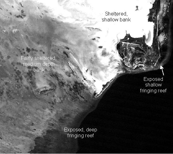
Principal physical environments of the Eastern Caicos Bank

Figure 1.3. Principal physical environments of the Eastern Caicos Bank

References

Clark, C.D., Ripley, H.T., Green, E.P., Edwards, A.J., and Mumby, P.J. (1997). Mapping and measurement of tropical coastal environments with hyperspectral and high spatial resolution data. International Journal of Remote Sensing 18: 237-242.

Congalton, R.G. (1991). A review of assessing the accuracy of classifications of remotely sensed data. Remote Sensing of Environment 37: 35-46.

Answers to Questions

The SPOT XS subscene is 550 pixels wide and 600 pixels long. If you put the cursor on the last (bottom right) pixel the status bar indicates you are on pixel 550, 600. Alternatively if you select the whole image with <Ctrl>+A and then select Edit GoTo you will see that the Selection Size: is 550 columns (DX:) and 600 rows (DY:). Each pixel is 23 x 23 m so the image is 12.65 km across (west to east) and 13.8 km long (north to south).
Red. This is because the sea tends to reflect more strongly in the green and (where shallow) in the red part of the spectrum (displayed through the blue and green guns respectively) than the land. Whilst the land tends to reflect much more strongly in the infra-red than the sea. Thus in the false colour composite the land appears dark on the blue and green guns but bright on the red gun. By contrast, deep sea areas are only bright on the blue gun, and shallow sea areas are bright on the blue and green guns (thus appearing cyan on the colour composite).
The runway is on the northern side of the main (south) part of South Caicos, running west to east between approximate column and row (x, y) coordinates 205, 415 and 300, 430. It is thus approximately 95 pixels long or about 2.2 km long.
Brown algae; because the area is close to the rocky shoreline and the habitat appears similar to that at 375, 118.
Dense seagrass; because it is a very homogeneous very dark patch with distinct boundaries which appears similar to the dense seagrass patch identified at 237, 112.
Less dense seagrass; it has a similar texture and boundaries to the dense seagrass but appears less dark.
An elkhorn coral (Acropora palmata) stand; because it appears similar in tone to the stand identified on Dove Cay at coordinates 334, 366 and is on the high wave-energy seaward end of Long Cay.
A small blowout in the seagrass bed; it looks similar to the blowout identified at coordinates 256, 146 but seems to have more seagrass or seagrass detritus lying on its bottom as it is darker.

APPENDIX 1.1

Landsat Thematic Mapper (TM) sensor

The Landsat Thematic Mapper (TM) has been operational since 1984 following the launch of Landsat-4. The spatial resolution for the sensor is 30 m except for Band 6 which measures emitted thermal infra-red radiation and has a resolution of 120 m. The radiometric resolution is 8 bits (256 grey levels). The swath width for the sensor is 185 km. At present (1995) the Thematic Mapper is only operational on Landsat-5 having failed on Landsat-4 in August 1993.

The spectral characteristics of the Landsat TM bands are as follows:-

TM Band	Colour	Wavelengths (nm)	Uses
1	Blue	450 - 520	Good water penetration; useful for mapping shallow coastal water. Strong vegetation absorbance; good for differentiating soil from vegetation, and deciduous from coniferous vegetation.
2	Green	520 - 600	Designed to measure visible green reflectance peak of vegetation for vigour assessment. Also useful for sediment concentrations in turbid water.
3	Red	630 - 690	Strongly absorbed by chlorophyll; an important band for vegetation discrimination. Also good for detecting ferric (red coloured) pollution.
4	Near Infra-red	760 - 900	Very strong vegetation reflectance; useful for determining biomass. High land/water contrast so good for delineating water bodies/coastlines.
5	Short Wave Infra-red	1550 - 1750	Moisture sensitive; indicative of vegetation moisture content and soil moisture.
6	Thermal Infra-red	10,400 - 12,500	Used in vegetation stress analysis, soil moisture discrimination, and thermal mapping.
7	Short Wave Infra-red	2080 - 2350	Good for discriminating rock types.

Images are produced by reflecting the radiance from 30 m wide scan lines on the Earth's surface to detectors on board the satellite using an oscillating mirror. Each scan line is 185 km long (thus the swath width or width of ground covered by the sensor in one overpass is 185 km). The Instantaneous Field of View (IFOV) of the sensor (roughly equivalent to the spatial resolution) is a 30 x 30 m square on the Earth's surface except for the thermal infra-red Band 6 where it is 120 x 120 m. Each pixel in a TM digital image is thus a measurement of the brightness of the radiance from a 30 x 30 m square on the Earth's surface.

Because the satellite is moving so fast over the Earth's surface, it has to scan 16 lines at a time or 4 lines at a time for Band 6 (thus covering 480 m along track). Since the TM sensor measures the radiance in seven different wavebands at the same time, it thus has 6 x 16 + 4 = 100 detectors in total. Each detector converts the recorded irradiance into an electrical signal which is converted to an 8 bit number (256 grey levels). The radiometric resolution of the TM sensor is thus 4 times that of the Landsat Multi-Spectral Scanner.

The image size is 185 km across by 172 km along-track; equivalent to 5760 lines by 6928 pixels. With seven wavebands each scene thus consists of about 246 Mbytes of data!

APPENDIX 1.2

SPOT

SPOT (Satellite Pour l'Observation de la Terre) is a remote sensing satellite developed by the French National Space Centre (CNES - Centre National d' Études Spatials) in collaboration with Belgium and Sweden. SPOT-1 was launched in February 1986, SPOT-2 in January 1990, SPOT-3 in September 1993 (failed in November 1997), and SPOT-4 in March 1998.

The satellite carries two High Resolution Visible (HRV) sensors. The HRV sensor is a "pushbroom scanner" which can operate in either multispectral mode (3 wavebands) at 20 m resolution (XS), or in panchromatic mode (1 waveband) at 10 m resolution (XP or Pan). Radiometric resolution is 8 bits (256 grey levels) in multispectral mode and 6 bits (64 grey levels) in panchromatic mode. The swath width is 60 km per HRV sensor and images are supplied as 60 x 60 km scenes. The two HRV sensors overlap by 3 km giving a swath width of 117 km for the satellite as a whole. SPOT-4 has enhanced capabilities (see http://www.spotimage.fr/ for details).

The mirror which focuses the light reflected from the ground-track onto the detector array can be angled by ground control through ~ 27- allowing off-nadir viewing within a strip 475 km to either side of the ground-track. Using the mirror, stereoscopic imagery can be obtained by imaging a target area obliquely from both sides on successive passes. The mirror also allows target areas to be viewed repeatedly (revisited) on successive passes such that at the Equator an area can be imaged on 7 successive days, whilst at latitude 45- eleven revisits are possible.

The detectors are Charge Coupled Devices (CCDs)å which form a solid state linear array about 8 cm long. Each pixel across the scan line is viewed by an individual detector in the array so that in panchromatic mode there are 6000 detectors each viewing a 10 m square pixel, whilst in multispectral mode there are 3000 detectors each viewing a 20 m square pixel on the Earth's surface. The linear array is pushed forward over the Earth's surface by the motion of the satellite, hence the name "pushbroom scanner".

å CCDs are light sensitive capacitors which are charged up in proportion to the incident radiation and discharged very quickly to give an electrical signal proportional to the radiance recorded.

Orbital characteristics

1) Near-polar sun-synchronous orbit.

2) Altitude of 832 km.

3) Inclination of 98.7-.

4) Equatorial crossing time at 10:30 h.

5) Repeat cycle 26 days.

HRV sensor spectral characteristics (SPOT 1 to 3)

	Spectral band
XS	Multispectral (20 m)
Band 1	Green, 500-590 nm
Band 2	Red, 610-680 nm
Band 3	Near-IR, 790-890 nm
XP or Pan	Panchromatic (10 m)
Band 1	510-730 nm

Images in either multispectral mode (XS) or panchromatic mode (PAN) can be purchased.

APPENDIX 1.3

Compact Airborne Spectrographic Imager (CASI).

CASI is a pushbroom imaging spectrograph designed for remote sensing from small aircraft. It comprises a two-dimensional 578 x 288 array of CCD (Charge Coupled Device) detectors. It is light (55 kg) and can be mounted in an aicraft as small as a Cessna 172 (single-engine, four seats). A modified Cessna door in which the instrument can be mounted is available so that CASI can be mounted without making holes in the aircraft. It requires only 250 Watt of power and can be run off a light aircraft's power circuit in most cases. If not, it can be run off a heavy duty lead-acid battery. CASI is manufactured by ITRES Research of Calgary, Alberta, Canada.

The width of the array is 578 detectors which in imaging mode view a strip 512 pixels wide underneath the aircraft (the remaining 64 detectors being used for calibration purposes). The angle of view is 35- and the width of this strip and size of the pixels is determined by the height of the aircraft. At an altitude of 840 m (2750 feet) pixels are 1 m wide, at about 2500 m they are 3 m wide. The speed of the aircraft and scanning rate of the instrument are adjusted to make the pixels square. It can scan at up to 100 lines per second. The instrument is designed for spatial resolutions of 1-10 m. The 288 detectors per pixel allow up to 288 different spectral bands (channels) to be sampled across a spectral range of about 400-900 nm. The minimum bandwith is 1.8 nm. The radiometric resolution is up to 12 bits (4096 grey levels).

In imaging mode a set of up to 16 spectral bands are chosen and the instrument is programmed to record in these bands. A set of bands chosen for remote sensing of shallow water features on the Caicos Bank in the Caribbean is shown below. At 1 m resolution it was found feasible to record in only 8 wavebands because of the rate of data acquisition required, whilst at 3 m resolution it was possible to record in 16 wavebands. A 16 band marine bandsetting optimised for water penetration was used for flight-lines over water, and a 16 band terrestrial bandsetting optimised for mangrove and vegetation mapping was used over land. Band settings could be switched in flight. Locating pixels accurately for ground-truthing at this high spatial resolution requires a good differential global positioning system (DGPS).

In multispectrometer mode the instrument records in 288 different 1.8 nm wide bands for up to 39 look directions (pixels at a time) across the swath width. This allows detailed spectral signatures of pixels to be built up. The difficulty is in determined precisely where these pixels are and then ground-truthing them so that spectral signatures can be assigned to defined habitats.

Back to main page

Back to Module 7

USDOC | NOAA | NESDIS | CoastWatch