 |
 |
Module 7 |
| Caribbean Regional Node | ||
|
|
Module 7 |
| Caribbean Regional Node | ||
Information | Data | Software | Sites | Education | Feedback | News
 Lesson8.
Assessing Mangrove Leaf-Area Index (LAI) Using
Lesson8.
Assessing Mangrove Leaf-Area Index (LAI) Using
Casi Airborne Imagery
Aim of Lesson
To learn how to assess mangrove leaf-area index (LAI)
using Compact Airborne Spectrographic Imager (CASI) imagery.
Objectives
2. To learn how LAI data is derived from field measurements.
3. To prepare a Normalised Vegetation Difference Index (NDVI) of mangrove areas from the CASI imagery
4. To investigate the relationship between NDVI and LAI using UTM coordinate referenced field survey data and use this relationship to create an image of mangrove Leaf Area Index.
5. To use a palette to display mangrove LAI effectively.
6. To calculate net canopy photosynthetic production from LAI and thus obtain a crude estimate of the mangrove forest primary productivity.
This lesson relates to material covered in Chapters 13 and 17 of the Remote Sensing Handbook for Tropical Coastal Management and readers are recommended to consult these for further details of the techniques involved. This lesson describes an empirical approach to mapping mangrove leaf-area index (LAI) using Compact Airborne Spectrographic Imager (CASI) imagery. The mangrove was located on the island of South Caicos.
In the eastern Caribbean the limited freshwater run off of the low dry islands and the exposure of a large portion of the shoreline to intense wave action imposes severe limits on the development of mangroves. They typically occur in small stands at protected river mouths or in narrow fringes along the most sheltered coasts (Bossi and Cintron 1990). As a result most of the mangrove forests in this region are small. Nevertheless they occur in up to 50 different areas where they are particularly important for water quality control, shoreline stabilisation and as aquatic nurseries. Mangroves in the Turks and Caicos Islands are typical of this area but completely different to the large mangrove forests which occur along continental coasts and at large river deltas.
The Bilko for Windows image processing software
Familiarity with Bilko for Windows 2.0 is required to carry out this lesson. In particular, you will need experience of using Formula documents to carry out mathematical manipulations of images and Histogram documents to calculate the area of particular features on the imagery. A familiarity with the Microsoft Excel spreadsheet package is also desirable.
Image data
The Compact Airborne Spectrographic Imager (CASI) was mounted on a locally-owned Cessna 172N aircraft using a specially designed door with mounting brackets and streamlined cowling. An incident light sensor (ILS) was fixed to the fuselage so that simultaneous measurements of irradiance could be made. A Differential Global Positioning System (DGPS) was mounted to provide a record of the aircraft's flight path. Data were collected at a spatial resolution of 1 m2 in 8 wavebands (Table 8.1) during flights over the Cockburn Harbour and Nigger Cay areas of South Caicos, Turks and Caicos Islands (21o 30' N, 71o 30' W) in July 1995. Further details are given in Clark et al. (1997).
|
|
|
|
| 1 | Blue |
|
| 2 | Blue |
|
| 3 | Green |
|
| 4 | Green |
|
| 5 | Red |
|
| 6 | Red |
|
| 7 | Near Infrared |
|
| 8 | Near Infrared |
|
Geometrically and radiometrically corrected Compact Airborne Spectrographic Imager (CASI) data from bands 6 (red) and 7 (near infra-red) of the area around South Caicos island are provided for the purposes of this lesson as files CASIMNG6.DAT and CASIMNG7.DAT. These files are unsigned 16-bit integer files (integers between 0 and 65535). This means that there are two bytes needed per pixel rather than the one byte needed for the Landsat TM and SPOT XS images which are only 8-bit data. Mangrove areas have to be separated from non-mangrove areas and a mask used to set water pixels and non-mangrove land pixels to zero.
Field survey data
Three species of mangrove, the red mangrove Rhizophora mangle, the white mangrove Laguncularia racemosa, and the black mangrove Avicennia germinans grow with the buttonwood Conocarpus erectus in mixed stands along the inland margin of the islands fringing the Caicos Bank. The field survey was divided into two phases. Calibration data were collected in July 1995, accuracy data in March 1996. Species composition, maximum canopy height and tree density were recorded at all sites (Table 8.2). Species composition was visually estimated from a 5 m2 plot marked by a tape measure. Tree height was measured using a 5.3 m telescopic pole. Tree density was measured by counting the number of tree trunks at breast height. When a tree forked beneath breast height (~1.3 m) each branch was recorded as a separate stem (after English et al., 1994). The location of each field site was determined using a Differential Global Positioning System (DGPS) with a probable circle error of 2-5 m.
Table 8.2. A summary of the field survey data. Data were collected in two phases; the first in 1995 for the calibration of CASI imagery and the second in 1996 for accuracy assessment. The number of sites at which each type of data was collected during each phase are shown. Category "Other" refers to field survey data for three non-mangrove categories (sand, saline mud crust, Salicornia species).
|
|
||
|
|
|
|
| Species composition (%) |
81
|
121
|
| Tree height |
81
|
121
|
| Tree density |
81
|
121
|
| Canopy transmittance |
30
|
18
|
| Percent canopy closure |
39
|
20
|
| Other |
37
|
67
|
A habitat classification was developed for the mangrove areas of the Turks and Caicos using hierarchical agglomerative clustering with group-average sorting applied to the calibration data. The calibration data were 4th root transformed in order to weight the contribution of tree height and density more evenly with species composition (the range of data was an order of magnitude higher for density and height and would cluster accordingly). This identified seven classes which separated at a Bray-Curtis Similarity of 85% level of similarity (Figure 8.1). Categories were described in terms of mean species composition (percent species), mean tree height and mean tree density (Table 8.3). One category, Laguncularia dominated mangrove, was discarded because white mangrove was rare in this area - in both the calibration and accuracy field phases it was observed at only two locations. Three other ground cover types were recorded: (i) sand, (ii) saline mud crust, and (iii) mats of the halophytic succulents Salicornia perennis and S. portulacastrum. These nine habitat categories (six mangrove, three other) were used to direct the image classification of the CASI data and the collection of accuracy data in 1996.
Two useful ways of describing or modelling the canopy structure of a vegetated area are leaf area index (LAI, Box 8.1) and percent canopy closure. Both can be estimated from remotely sensed data, which is advantageous in areas where access is particularly difficult or when alternative methods are laborious and difficult to replicate properly over large areas.
Leaf area index
Many methods are available to measure LAI directly and are variations of either leaf sampling or litterfall collection techniques. These methods tend to be difficult to carry out in the field, extremely labour intensive, require many replicates to account for spatial variability in the canopy and are thus costly in terms of time and money. Consequently many indirect methods of measuring LAI have been developed (see references in Nel and Wessman, 1993). Among these are techniques based on gap-fraction analysis that assume that leaf area can be calculated from the canopy transmittance (the fraction of direct solar radiation which penetrates the canopy). This approach to estimating LAI uses data collected from beneath the mangrove canopy and was used here.
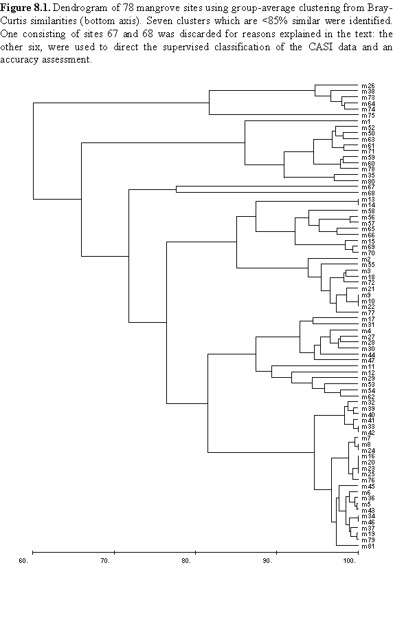
Table 8.3. Descriptions for each of the mangrove
habitat categories identified in Figure 8.1. N = number of calibration
sites in each category. Rhz = Rhizophora; Avn = Avicennia;
Lag = Laguncularia; Con = Conocarpus.
|
|
|
|
|
|
|||
|
|
|
|
|
|
|
||
| Conocarpus erectus |
|
|
|
|
|
|
|
| Avicennia germinans |
|
|
|
|
|
|
|
| Short, high density, Rhizophora mangle |
|
|
|
|
|
|
|
| Tall, low density, Rhizophora mangle |
|
|
|
|
|
|
|
| Short mixed mangrove, high density |
|
|
|
|
|
|
|
| Tall mixed mangrove, low density |
|
|
|
|
|
|
|
| Laguncularia dominated mangrove |
|
|
|
|
|
|
|
| Unclassified |
|
||||||
Box 8.1. Leaf area index (LAI).
LAI is defined as the single-side leaf area per unit ground area, and as such is a dimensionless number. The importance of LAI stems from the relationships which have been established between it and a range of ecological processes such as rates of photosynthesis, transpiration and evapotranspiration (McNaughton and Jarvis, 1983; Pierce and Running, 1988), and net primary production (Monteith, 1972; Gholz, 1982). Measurements of LAI have been used to predict future growth and yield (Kaufmann et al., 1982) and to monitor changes in canopy structure due to pollution and climate change. The ability to estimate leaf area index is therefore a valuable tool in modelling the ecological processes occurring within a forest and in predicting ecosystem responses.
Mangroves are intertidal, often grow in dense stands and have complex aerial root systems which make extensive sampling impractical with the difficulty of moving through dense mangrove stands and the general inaccessibility of many mangrove areas posing a major logistic problem. Luckily field measurements indicate that there is a linear relationship between mangrove LAI and normalised difference vegetation index (Ramsey and Jensen, 1995; 1996). NDVI can be obtained from remotely sensed data. This means that a relatively modest field survey campaign can be conducted to obtain LAI measurements in more accessible mangrove areas and these used to establish a relationship to NDVI using regression analysis. Once this relationship is known then NDVI values for the remainder of the mangrove areas can be converted to LAI.
Measurement of canopy transmittance and calculation of LAI
LAI is a function of canopy transmittance, the fraction of direct solar radiation which penetrates the canopy. Canopy transmittance is given by the ratio Ic/Io where Ic = light flux density beneath the canopy and Io = light flux density outside the canopy. LAI can then be calculated, and corrected for the angle of the sun from the vertical, using the formula
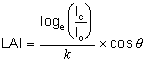
where LAI = leaf area index, q = sun zenith angle in degrees (this can be calculated from time, date and position), k = canopy light extinction coefficient, which is a function of the angle and spatial arrangement of the leaves. The derivation of this formula is given in English et al. (1994). For each field site loge(Ic/ Io) was calculated for 80 pairs of simultaneous readings of of Ic and Io around the position fix and averaged. A value for k of 0.525 was chosen as being appropriate to mangrove stands.
Measurements were taken on clear sunny days between 10:00 and 14:00 hours, local time. The solar zenith angle was judged to be sufficiently close to normal (i.e. perpendicular) two hours either side of noon for directly transmitted light to dominate the radiation spectrum under the canopy. At other times the sun is too low and diffuse light predominates. Photosynthetically active radiation (PAR) was measured using two MACAM ™ SD101Q-Cos 2p PAR detectors connected to a MACAM ™ Q102 radiometer. One detector was positioned vertically outside the mangrove canopy on the end of a 40 m waterproof cable and recorded Io. The other detector recorded Ic and was connected to the radiometer by a 10 m waterproof cable. If the mangrove prop roots and trunk were not too dense to prevent a person moving around underneath the canopy this detector (which was attached to a spirit level) was hand-held. If the mangroves were too dense then the Ic detector was attached to a 5.4 m extendible pole and inserted into the mangrove stand. The spirit level was attached to the end of the pole to ensure the detector was always vertical. All recordings of Ic were taken at waist height, approximately 0.8 m above the substrate.
Lesson Outline
Creating a Normalized Difference Vegetation Index (NDVI) image
Since NDVI is calculated using near infra-red and red bands there were four options for calculating NDVI from the CASI data with combinations of Bands 5 to 8 (Table 8.4). The relationships between NDVI calculated from Bands 8 and 5 or from Bands 8 and 6, and values of LAI estimated from in situ measured canopy transmittance, were not significant. However, there were significant relationships when LAI was regressed against NDVI calculated either from Bands 7 and 6 or 7 and 5 (Table 8.4). NDVI derived from Bands 6 and 7 was deemed most appropriate for the prediction of LAI because (i) it accounts for a much higher proportion of the total variation in the dependent variable, and (ii) the accuracy with which the model predicts the dependence of LAI on NDVI is higher (the standard error of estimate is lower). This is why CASI bands 6 and 7 have been selected for this exercise.
Visually inspect the two images, stretching as necessary to see them clearly. Note that with a spatial resolution of around 1 m, there is quite a lot of texture visible in the mangrove canopy.
Using both images and the Edit,GoTo function answer the following question.
Question: 8.1. Is
the mangrove vegetation thicker and the canopy closure greater at UTM coordinates
236520 E, 2379938 N than at 236600 E, 2379945 N, or is the reverse true?
Explain the reasons behind your conclusion. [Both coordinate positions
are near the bottom of the image]. Answers
|
|
|
|
|
|
|
| (Band 8 - Band 5)/(Band 8 + Band 5) | 0.22 | 0.19 | 0.05 | NS | 1.93 |
| (Band 8 - Band 6)/(Band 8 + Band 6) | 0.12 | 3.68 | 2.29 | NS | 2.18 |
| (Band 7 - Band 6)/(Band 7 + Band 6)* | 0.77 | 0.31 | 9.76 | <0.001 | 0.99 |
| (Band 7 - Band 5)/(Band 7 + Band 5)* | 0.43 | 1.81 | 5.71 | <0.001 | 1.69 |
The next step is to calculate a Normalised Difference
Vegetation Index image (Box 8.2) from the CASI bands 6 and 8. In a real
life situation you would check all possible band-pair combinations and
see which was best for predicting LAI. Here we will just work with the
band pair which we found to give best results.
Box 8.2 The use of vegetation indices in the remote sensing of mangroves
Vegetation indices are complex ratios involving mathematical transformations of spectral bands. As such, vegetation indices transform the information from two bands or more into a single index. For example, the normalised difference vegetation index or NDVI is a common vegetation index calculated from red and infra-red bands:
NDVI = ![]()
The results of this calibration exercise are summarised in Table 8.6 below but the calculation of average NDVI for two sites has been left for you to do. Site 72 has short sparse mangrove and thus a relatively low LAI, whilst site 79 is on the edge of a reasonably dense stand of mangrove and has a much higher LAI. Both sites are towards the south-east of the image.
Important. The Edit, GoTo function tries to get you to the nearest pixel to the coordinates entered; sometimes the coordinates you enter may be half way between two pixels. Such is the case for the central pixel of Site 79. Note that the Edit, GoTo puts you on 236693, 2380129 so you need to move down one pixel to get to the central pixel which should have the value 0.6065. Use the <Ctrl>+<Down> arrow key.
[Enter values to 4 decimal places].
|
Central pixel: X: 236700, Y: 2379827 |
Central pixel: X: 236693, Y: 2380128 |
|||||
Question: 8.2. What are the average NDVIs at site 72 and 79 (to two decimal places)? Answers
|
|
|
|
||
|
|
|
|
|
|
|
31
|
237118
|
2378993
|
0.70
|
6.61
|
|
33
|
237105
|
2378990
|
0.75
|
7.32
|
|
34
|
237094
|
2378986
|
0.81
|
8.79
|
|
36
|
237114
|
2379026
|
0.63
|
6.62
|
|
37
|
237103
|
2379022
|
0.78
|
7.83
|
|
39
|
237087
|
2379071
|
0.79
|
6.17
|
|
40
|
237092
|
2379075
|
0.73
|
6.87
|
|
43
|
237115
|
2379080
|
0.69
|
6.96
|
|
44
|
237070
|
2379373
|
0.47
|
2.53
|
|
47
|
237038
|
2379376
|
0.75
|
6.61
|
|
52
|
237026
|
2379456
|
0.28
|
2.52
|
|
53
|
237005
|
2379491
|
0.64
|
5.04
|
|
54
|
236989
|
2379500
|
0.63
|
5.35
|
|
56
|
237008
|
2379445
|
0.61
|
4.76
|
|
59
|
237020
|
2379567
|
0.29
|
2.33
|
|
61
|
236997
|
2379540
|
0.42
|
4.34
|
|
62
|
236978
|
2379547
|
0.47
|
4.96
|
|
64
|
236932
|
2379588
|
0.24
|
1.93
|
|
65
|
236890
|
2379549
|
0.47
|
5.82
|
|
66
|
236872
|
2379554
|
0.42
|
3.74
|
|
67
|
236759
|
2379649
|
0.49
|
6.58
|
|
68
|
236731
|
2379664
|
0.43
|
3.89
|
|
71
|
236718
|
2379777
|
0.59
|
5.59
|
|
72
|
236700
|
2379827
|
1.64
|
|
|
73
|
236723
|
2379825
|
0.29
|
2.33
|
|
75
|
236668
|
2379932
|
0.19
|
1.99
|
|
78
|
236579
|
2380039
|
0.35
|
2.03
|
|
79
|
236693
|
2380128
|
5.83
|
|
|
80
|
236703
|
2380141
|
0.61
|
2.95
|
|
81
|
236728
|
2380128
|
0.47
|
5.05
|
Regression of LAI on NDVI
You now need to carry out the regression of Leaf Area Index on NDVI to allow you to map LAI from the CASI imagery. Luckily there is a simple linear relationship between LAI and NDVI defined by the regression equation:
LAI = intercept + slope x NDVI
Question: 8.3. What is the intercept and slope of the regression of LAI on NDVI (to 4 decimal places)? Answers
|
|
|
|
|
|
|
|
|
|
|
|
|
|
|
|
|
|
Knowing the relationship between NDVI on the image and LAI measured in the field we can now make an 8-bit (byte) image of Leaf Area Index by applying a Formula document to convert NDVI to LAI. From the graph of LAI against NDVI we know that the maximum LAI we will find is about 10. To spread our LAI measure over more of the display scale (0-255) whilst making it easy to convert pixel values to LAI we can multiply by 10. This will mean that LAI values up to 2 will map to pixel values between 1 and 20, and so on (see table to right). Thus a pixel value of 56 in the output image will indicate an LAI of 5.6.
The Formula document will thus need to be something like this:
( intercept + slope * @x ) * 10 ;
where you substitute the values you obtained in the regression analysis for the intercept and slope and @x is the NDVI image.
Use File, New to open a new Formula document and enter a formula (see above) to carry out the conversion of NDVI to LAI (use constant statements as appropriate to set up input values and make the formula easy to understand). Use the Formula document Options! to make sure the output image is Byte (8 bits)and then Copy the formula and Paste it to the connected images. The resultant image will be dark because the highest pixel value is only 100. To see the distribution of mangrove with different levels of LAI, open the Palette document LAI.PAL whilst the LAI image is the active document. The palette will be automatically applied to the image [assuming Apply is checked in the File, Open dialog box] and displays each of the five ranges of LAI in a different shade of green to green-brown. Note that mangrove areas with a Leaf Area Index greater than 8 are very rare.
Check: Note the value of the pixel at x, y (column, row) coordinate 324, 1167 in the MANGNDVI.DAT image. It should be 0.8333. Use a calculator to work out what its LAI value should be using your equation. It should be 7.8 and thus the pixel value at 324, 1167 on the LAI image should be 78. If it isn't something has gone wrong.
Question: 8.4. What percentage of the image area is mangrove? Answers
From the histogram header one can see that the image is 500 pixels wide and 1325 pixels long. Knowing that each pixel is 1.0 m wide and 1.1 m long, calculate the area of the whole image in hectares (1 ha = 100 x 100 m = 10,000 m?). Complete Table 8.7 with all values recorded to one decimal place, then answer the questions below.
Question: 8.5. What is the area of the whole image in hectares (to the nearest hectare)? Answers
8.6. What is the total area of mangrove in hectares ( to the nearest hectare)?
8.7. How many hectares of mangrove have an LAI > 6 and what proportion of the total mangrove area does this represent?
|
|
|
|
|
|
|
|
||
|
|
|
||
|
|
|
||
|
|
|
||
|
|
|
||
|
|
|
0.05
|
|
|
Total area of mangrove
|
|||
|
Total area of image
|
|||
Estimation of net canopy photosynthetic production (PN)
The approximate net photsynthetic production of the whole mangrove canopy per m? of ground area over a day can be described by the following equation:
PN = A x d x LAI
where A = average rate of photsynthesis (gC m-2 leaf area hr-1) for all leaves in the canopy, d = daylength (hr), and LAI is the leaf area index already estimated for each pixel (English et al. 1994). For mangroves in high soil salinities in the dry season a reasonable estimate for A = 0.216 gC m-2 hr-1 and daylength in the Turks and Caicos is on average about 12 hours. Using this relationship we can make a rough estimate of the net photosynthetic production in each LAI class, indeed, if one had good field data on the average rate of photosynthesis (A) one might in theory make an image where pixel values related to PN. For the purpose of this lesson we are just going to make a crude estimate of the number of tonnes of carbon fixed per hectare each year (tC ha-1 year-1) by the mangrove area with an LAI of 6-8.
Question: 8.8. What do you estimate the daily net photosynthetic production of the mangroves with LAI 6-8 in gC m-2? What is this as an annual production in units of tC ha-1 year-1? [Show your working]. Answers
8.9. How many tonnes of carbon are fixed per year by these mangroves (LAI 6-8) in the area of the image?
Bossi, R. and Cintron, G. 1990. Mangroves of the Wider Caribbean: toward Sustainable Management. Caribbean Conservation Association, the Panos Institute, United Nations Environment Programme.
Clark, C.D., Ripley, H.T., Green, E.P., Edwards, A.J. and Mumby, P.J. 1997. Mapping and measurement of tropical coastal environments with hyperspectral and high spatial resolution data. International Journal of Remote Sensing 18: 237-242.
Clough, B.F., Ong, J.E. and Gong, G.W., 1997. Estimating leaf area index and photosynthetic production in mangrove forest canopies. Oecologia. in press.
English, S., Wilkinson, C. and Baker, V. 1994. Survey Manual for Tropical Marine Resources. Australian Institute of Marine Science, Townsville. 368 pp.
Gholz, H.L., 1982. Environmental limits on above-ground net primary production, leaf area and biomass in vegetation zones of the Pacific Northwest. Ecology 63: 469-481.
Kaufmann, M.R., Edminster, C.B., and Troendle, C., 1982. Leaf area determinations for subalpine tree species in the central Rocky Mountains. U.S. Dep. Agric. Rocky Mt. For. Range. Exp. Stn. Gen. Tech. Rep., RM-238.
McNaughton, K.G. and Jarvis, P.G., 1983. Predicting effects of vegetation changes on transpiration and evaporation. In: Water Deficits and Plant Growth. Vol. 7. Ed. Kozlowski, T.T. Academic Press, London, UK. pp. 1-47.
Monteith, J.L., 1972. Solar radiation and productivity in tropical ecosystems. Journal of Applied. Ecology 9: 747-766.
Nel, E.M. and Wessman, C.A., 1993. Canopy transmittance models for estimating forest leaf area index. Canadian Journal of Forest Research 23: 2579-2586.
Pierce, L.L. and Running, S.W. 1988. Rapid estimation of coniferous forest leaf area index using a portable integrating radiometer. Ecology69: 1762-1767.
Ramsey, E.W. and Jensen, J.R. 1995. Modelling mangrove canopy reflectance by using a light interception model and an optimisation technique. In: Wetland and Environmental Applications of GIS, Lewis, Chelsea, Michigan, USA.
Ramsey, E.W. and Jensen, J.R. 1996. Remote sensing of
mangrove wetlands: relating canopy spectra to site-specific data. Photogrammetric
Engineering and Remote Sensing 62 (8): 939-948.
|
Central pixel: X: 236700, Y: 2379827 |
Central pixel: X: 236693, Y: 2380128 |
|||||
|
|
|
|
|
|
|
|
|
|
|
|
|
|
|
|
|
|
|
|
|
|
|
|
|
|
|
|
|
|
|
|
44.69
|
|
|
|
|
8.60
|
|
|
|
|
8.79
|
|
|
|
|
24.72
|
|
|
|
|
13.15
|
|
|
|
|
0.05
|
|
|
Total area of mangrove
|
55.31
|
|
|
|
Total area of image
|
100.00
|
|
|
Example Formula documents:
1) To calculate NDVI:
# Formula to calculate NDVI [Lesson 8]
# @1 = near infra-red image (in this case CASIMNG7.DAT)
# @2 = red image (in this case CASIMNG6.DAT)
# The output image needs to be Float (32 bit)
CONST Infrared = @1 ;
CONST Red = @2 ;
(Infrared - Red) / (Infrared + Red)
;
2) To calculate LAI:
# Formula to calculate LAI from NDVI for CASI mangrove image [Lesson 8]
# LAI has been regressed against NDVI and the intercept and slope of the linear
# relationship have been found. These will be set up as constants.
# The formula assumes MANGNDVI.DAT is @1 and the blank image is @2.
# The output image is an 8-bit GIF file where pixel value = LAI * 10.
CONST intercept = -0.3123 ;
CONST slope = 9.7566 ;
CONST ScaleFactor = 10 ;
( intercept + slope * @1 ) * ScaleFactor ;
 |
Back to main page | Back to Module 7 | USDOC | NOAA | NESDIS | CoastWatch |