 |
 |
Module 7 |
| Caribbean Regional Node | ||
|
|
Module 7 |
| Caribbean Regional Node | ||
Information | Data | Software | Sites | Education | Feedback | News
 Lesson
4. Crude Bathymetric Mapping Using Landsat TM Satellite Imagery
Lesson
4. Crude Bathymetric Mapping Using Landsat TM Satellite Imagery
Aim of Lesson
To learn how bathymetry can be mapped crudely from digital
imagery and the limitations of the results.
Objectives
2. To use deep water pixels to determine maximum DN values returned over deep water for Landsat TM bands 1 to 4.
3. To derive maximum depth of penetration estimates for Landsat TM bands 1 to 4 for the Caicos Bank using UTM coordinate referenced field survey data of depths.
4. To combine these data to define depth of penetration (DOP) zones, assign pixels to these zones, and display a very crude bathymetric map of these depth zones.
5. To refine this map by interpolation using information on maximum and minimum DN values in each DOP zone and create an image where pixel values correspond to depth.
6. To create a palette to display depth contours.
7. To investigate the limitations of the method.
This lesson relates to material covered in Chapter 15 of the Remote Sensing Handbook for Tropical Coastal Management and readers are recommended to consult this for further details of the techniques involved. This lesson describes an empirical approach to mapping bathymetry using Landsat Thematic Mapper imagery of the Caicos Bank.
Depth information from remote sensing has been used to augment existing charts (Bullard, 1983; Pirazolli, 1985), assist in interpreting reef features (Jupp et al., 1985) and map shipping corridors (Benny and Dawson, 1983). However, it has not been used as a primary source of bathymetric data for navigational purposes (e.g. mapping shipping hazards). The major limitations are inadequate spatial resolution and lack of accuracy. Hazards to shipping such as emergent coral outcrops or rocks are frequently be much smaller than the sensor pixel and so will fail to be detected.
Among satellite sensors, the measurement of bathymetry can be expected to be best with Landsat TM data because that sensor detects visible light from a wider portion of the visible spectrum, in more bands, than other satellite sensors. Landsat bands 1, 2 and 3 are all useful in measuring bathymetry: so too is band 4 in very shallow (<1 m), clear water over bright sediment (where bands 1-3 tend to be saturated). Bands 5 and 7 are completely absorbed by even a few cm of water and should therefore be removed from the image before bathymetric calculations are performed.
This lesson will help you understand the importance of water depth in determining the reflectance of objects on the seabed and prepare you for understanding Lesson 5 which deals with how one attempts to compensate for these effects.
The Bilko for Windows image processing software
Familiarity with Bilko for Windows 2.0 is required to carry out this lesson. In particular, you will need experience of using Formula documents to carry out mathematical manipulations of images. Spreadsheet skills are also essential to benefit fully from the lesson. Instructions for spreadsheet manipulations are given for Excel and should be amended as appropriate for other spreadsheets.
Image data
The image you will be using was acquired by Landsat 5 TM on 22nd November 1990 at 14.55 hours Universal Time (expressed as a decimal time and thus equivalent to 14:33 GMT). The Turks & Caicos are on GMT - 5 hours so the overpass would have been at 09:33 local time. You are provided with bands 1 (blue), 2 (green), 3 (red) and 4 (near-infrared) of part of this image as the files TMBATHY1.GIF, TMBATHY2.GIF, TMBATHY3.GIF, and TMBATHY4.GIF. These images are of DN values but have been geometrically corrected. The post-correction pixel size is 33 x 33 m and each image is 800 pixels across and 900 pixels along-track.
Question: 4.1. How many kilometres wide and long is the image? Answers
The fundamental principle behind using remote sensing to map bathymetry is that different wavelengths of light will penetrate water to a varying degree. When light passes through water it becomes attenuated by interaction with the water column. The intensity of light remaining (Id) after passage length p through water, is given by:
![]() Equation 4.1
Equation 4.1
where I0 = intensity of the incident light and k = attenuation coefficient, which varies with wavelength. Equation 4.1 can be made linear by taking natural logarithms:
![]() Equation 4.2
Equation 4.2
Red light attenuates rapidly in water and does not penetrate further than about 5 m in clear water. By contrast, blue light penetrates much further and in clear water the seabed can reflect enough light to be detected by a satellite sensor even when the depth of water approaches 30 m. The depth of penetration is dependent on water turbidity. Suspended sediment particles, phytoplankton and dissolved organic compounds will all effect the depth of penetration (and so limit the range over which optical data may be used to estimate depth) because they scatter and absorb light, thus increasing attenuation.
Depth of penetration zones method (modified from Jupp, 1988)
There are two parts to Jupp's method i) the calculation of depth of penetration zones or DOP zones, (ii) the interpolation of depths within DOP zones.
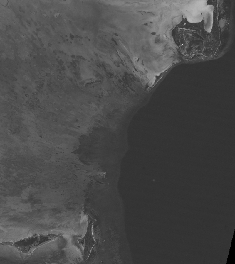
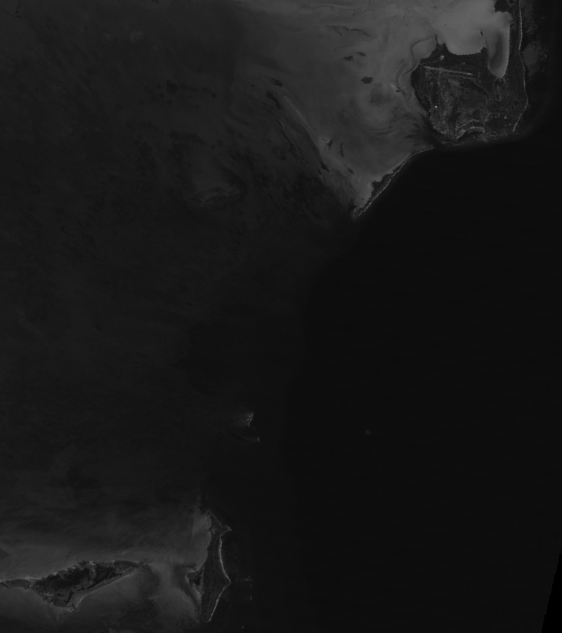
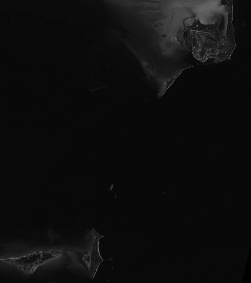
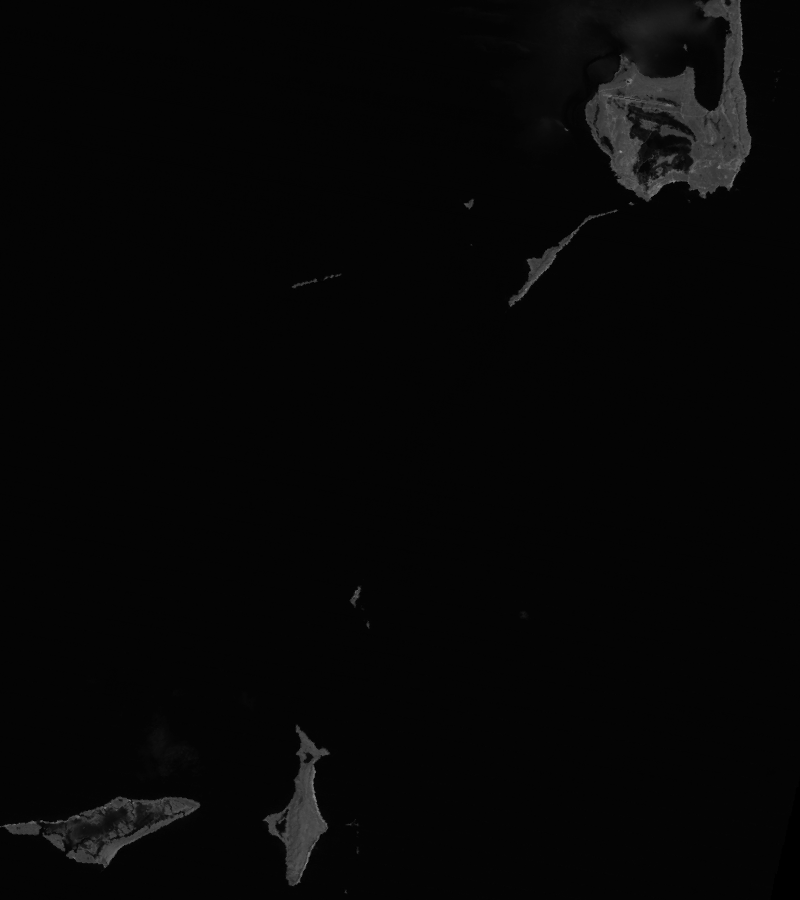
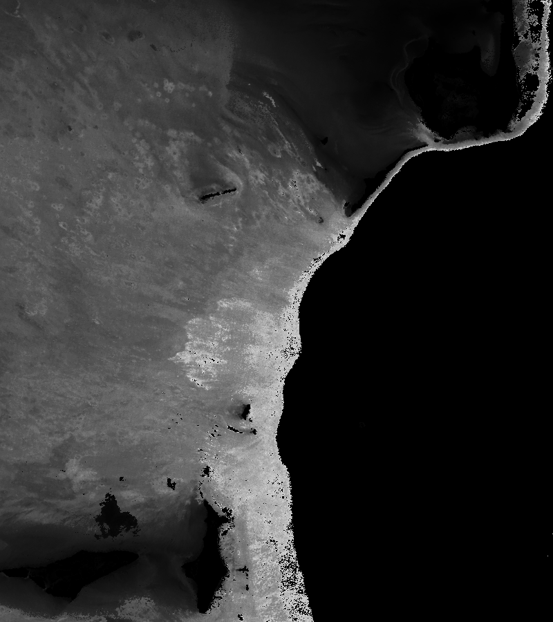
The coefficient of attenuation k depends on wavelength. Longer wavelength light (red in the visible part of the spectrum) has a higher attenuation coefficient than short wavelengths (blue). Therefore red light is removed from white light passing vertically through water faster than is blue. There will therefore be a depth at which all the light detected by band 3 (visible red, 630-690 nm)) of the Landsat TM sensor has been attenuated (and which will therefore appear dark in a band 3 image). However not all wavelengths will have been attenuated to the same extent - there will still be shorter wavelength light at this depth which is detectable by bands 2 and 1 of the Landsat TM sensor (visible green, 520-600 nm; and visible blue, 450-520 nm respectively). This is most easily visualised if the same area is viewed in images consisting of different bands (Figure 4.1). The shallowest areas are bright even in band 4 but deeper areas (> about 15 m) are illuminated only in band 1 because it is just the shorter wavelengths which penetrate to the bottom sufficiently strongly to be reflected back to the satellite.
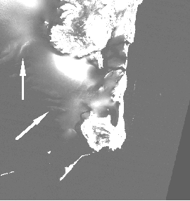
Figure 4.1. Band 1 and 4 Landsat TM images (DN) of the area around South Caicos. Deeper areas are illuminated by shorter wavebands. There is deep (30 - 2500 m) water in the bottom right hand corner of the images - this is not completely dark because some light is returned to the sensor over these areas by specular reflection and atmospheric scattering. Band 1 illuminates the deep fore reef areas (as indicated by the arrows). The edge of the reef or `drop-off' can be seen running towards the top right hand corner of the band 1 image. In areas of shallow (<1 m) clear water over white sand band 4 reveals some bathymetric detail (as indicated by the arrows).
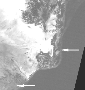
Landsat TM Band 1 Landsat TM Band 4
The attenuation of light through water has been modelled by Jerlov (1976) and the maximum depth of penetration for different wavelengths calculated for various water types. Taking Landsat MSS as an example, it is known that green light (band 1, 0.50-0.60 m m) will penetrate to a maximum depth of 15 m in the waters of the Great Barrier Reef, red light (band 2, 0.60-0.70 m m) to 5 m, near infra-red (band 3, 0.70-0.80 m m) to 0.5 m and infra-red (band 4, 0.80-1.1 m m) is fully absorbed (Jupp, 1988).
Thus a "depth of penetration" zone can be created for each waveband (Figure 4.2). One zone for depths where green but not red can penetrate, one for where red but not near infra-red can penetrate, and one for where near-infrared (band 3) but not infra-red (band 4) can penetrate. Thus for the Landsat MSS example over clear Great Barrier Reef water three zones could be determined: 5-15 m, 0.5-5 m and surface to 0.5 m depth.
The method of Jupp (1988) has three critical assumptions:
2. Water quality (and hence k) does not vary within an image.
3. The colour (and therefore reflective properties) of the substrate is constant.
Question: 4.2. Which assumption do you think is most likely not to be satisfied in the clear waters over the Caicos Bank? Answers
UTM coordinate referenced field survey depth measurements for 515 sites on the Caicos Bank are provided in the Excel spreadsheet file DEPTHS.XLS. This includes the date, time, UTM coordinates from an ordinary or Differential Global Positioning System (GPS or DGPS), depth in metres (to nearest cm) measured using a hand-held echo-sounder, and DN values recorded in Landsat Thematic Mapper bands 1 to 4 at each coordinate (obtained using ERDAS Imagine 8.2 software).
The Tidal Prediction by the Admiralty Simplified Harmonic Method NP 159A Version 2.0 software of the UK Hydrographic Office was used to calculate tidal heights during each day of field survey so that all field survey depth measurements could be corrected to depths below datum (Lowest Astronomical Tide). [Admiralty tide tables could be used if this or similar software is not available]. The predicted tidal height at the time of the satellite overpass at approximately 09.30 h local time on 22 November 1990 was 0.65 m (interpolated between a predicted height of 0.60 m at 09.00 h and one of 0.70 m at 10.00 h). This height was added to all measured depths below datum to give the depth of water at the time of the satellite overpass.
|
|
zi |
|
|
|
|
|
|
|
|
|
|
|
|
Lesson Outline
Step 1. Calculating depth of penetration zones
The first task is to find out what the maximum DN values of deep water pixels are for bands 1-4 of the Landsat TM image. At the same time we will note the minimum values. If the image had been radiometrically and atmospherically corrected, the reflectance from deep water would be close to zero but because it has not although no light is being reflected back from the deep ocean the sensors will be recording significant DN values because of atmospheric scattering, etc. Knowing the highest DN values over deep water provides us with a baseline that we can use to determine the depth at which we are getting higher than background reflectance from the seabed. For each waveband, if DN values are greater than the maximum deep water values then we assume the sensor is detecting light reflected from the seabed.
|
|
||||
|
|
|
|
|
|
| Maximum deepwater DN value (Ldeep max) | ||||
| Minimum deepwater DN value (Ldeep min) | ||||
| Mean deepwater DN value (Ldeep mean) | ||||
The next stage is to use UTM coordinate referenced field survey data to estimate the maximum depths of penetration for each waveband. This can be done by inspecting the file DEPTHS.XLS which contains details of measured depths and DN values for 515 field survey sites. The survey sites have been sorted on depth with the deepest depths first. Table 4.1 lists the maximum depths of penetration recorded by Jupp (1988) for bands 1-4 of Landsat TM which gives us a starting point for searching for pixels near the maximum depth of penetration.
Note: The (D)GPS derived UTM coordinates for the depth measurements had positional errors in the order of 18-30 m for GPS coordinates and 2-4 m for DGPS ones. The Landsat TM pixels are 33 x 33 m in size. The reflectances recorded at the sensor are an average for the pixel area with contributions from scattering in the atmosphere. There is thus spatial and radiometric uncertainty in the data which needs to be considered. At the edge of the reef depth may change rapidly and spatial uncertainty in matching pixel DN values to depths is likely be most acute.
| [Depths in metres] |
|
|||
|
|
|
|
|
|
| Depth of deepest pixel with DN > Ldeep max |
|
|
||
| Depth of shallowest pixel with DN <= Ldeep max |
|
|
||
| Average depth of boundary pixels with DN values > Ldeep max |
|
|
||
| Average depth of boundary pixels with DN values = Ldeep max |
|
|
||
| Estimated maximum depth of penetration (zi) |
|
|
||
For Landsat TM1 you will find that the average depth of those pixels which have DN values > Ldeep max is slightly less than that for pixels with values of 56-57. Given the small sample size and spatial and other errors this is understandable. The maximum depth of penetration for TM1 (z1) presumably lies somewhere between these two depths and for our protocol we will take the average of the two depths as being our best estimate.
Repeat part of the exercise for band 2 (the values have been pre-sorted for you) and enter the appropriate values into Table 4.3.
Inspect the spreadsheet to see how the values were calculated for bands 3 and 4. Note that the estimate of z4 is unlikely to be very accurate, however, study of the near-infrared image does indicate significant reflectance in very shallow water over white sand.
Figure 4.2. Diagram to show the rationale behind Jupp's depth of penetration (DOP) zones.
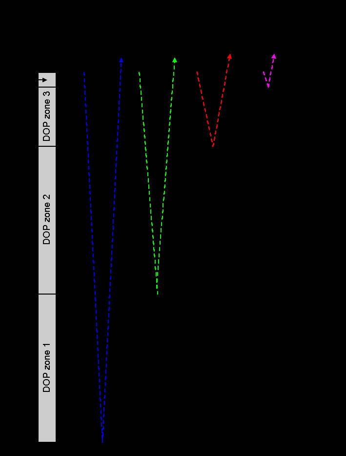
Table 4.4. A decision tree to assign pixels to depth zones.
|
|
|
|
|
|
|
| Deepwater maximum DN |
|
|
|
|
|
| If DN value (Li) of pixel | <= 57 | <= 16 | <= 11 | <= 5 | then depth > 20.8 m |
| If DN value (Li) of pixel | >57 | <= 16 | <= 11 | <= 5 | then depth = 13.5-20.8 m (zone 1) |
| If DN value (Li) of pixel | >57 | >16 | <= 11 | <= 5 | then depth = 4.2-13.5 m (zone 2) |
| If DN value (Li) of pixel | >57 | >16 | >11 | <= 5 | then depth = 1.0-4.2 m (zone 3) |
| If DN value (Li) of pixel | >57 | >16 | >11 | >5 | then depth = 0-1.0 m (zone 4) |
If none of these conditions apply, then pixels are coded to 0. A few pixels may have higher values in band 2 than band 1, which should not happen in theory. These will also be coded to zero and filtered out of the final depth image.
To implement this decision tree you will need to set up a Formula document with a series of conditional statements. This is primarily a lesson in remote sensing not computing so I have prepared one for you which creates four new images, showing the four DOP zones.
Open the formula document file DOPZONES.FRM and study how it works. Essentially each formula creates a mask where pixels in a DOP zone are coded to one and pixels outside the depth zone are coded to zero. Note that for DOP zone 4, defined by near-infrared penetration, that the land areas will also be coded to one; a land mask image (LANDMSK4.GIF) is thus be needed to separate land from very shallow water. Make sure the formula document Options! menu is set so that the output images are the Same as @1.
Copy the formula document and Paste it to the connected images to create the four DOP zone mask images.
Close the connected images window.
Inspect the four DOP zone mask images having stretched them (Auto Linear). Note the thin band of DOP zone 1 around the edge of the Caicos Bank (becoming broader as one moves south) but huge extent of DOP zone 2.
Connect the four DOP zone images, using the connect toolbar to make sure that DOP zone 1 is @1, DOP zone 2 is @2, etc.
4.7. What habitat do you think is causing the deep water anomalies (around coordinates 769, 120 and 776, 133)? [Hint: Use the Landsat TM1 image to help identify the cause.]
Activity: The final stage for finishing your DOP zone bathymetric image is to smooth out odd pixels. To do this run a 3 x 3 median filter over the image (Image, Filter, Median). Note the improved look to the image as a result of smoothing. Save the image as DOP4ZONE.GIF and then close it. Close the connected images window and Save the DOP zones 1-4 mask images as DOPMASK1.GIF, DOPMASK2.GIF, DOPMASK3.GIF and DOPMASK4.GIF.
Step 2. Interpolation of DOP zones
Calculating DOP zones does not assign a depth to each pixel, instead it assigns a pixel to a depth range (e.g. 13.5-20.8 m). Step two of Jupp's method involves interpolating depths for each pixel within each DOP zone. We will only work with DOP zone 2.
In DOP zone 2, the DN value of any submerged pixel in TM band 2 (L2) can be expressed as:
![]() Equation 4.3
Equation 4.3
where L2 deep mean is the average deep water pixel value for TM band 2 calculated in Table 4.2, L2 surface is the average DN value at the sea-surface (i.e. with no attenuation in the water column), k2 is the attenuation coefficient for TM band 2 wavelengths through the water column, and z is the depth. Thus for a particular bottom type the DN value can vary between a minimum which is the mean deep water DN, and a maximum which is the DN which would be obtained if that bottom type was at the surface and no attenuation was occurring. In between the maximum depth of penetration for TM band 2 (z2) and the surface, the DN value is purely a function of depth (z), with the rate of decrease in DN with depth being controlled by the attenuation coefficient for band 2 (k2).
Equation 4.3 can be rewritten as:
![]() Equation 4.4
Equation 4.4
If we define X2 as follows: ![]()
we can get rid of the exponential thus:
![]() Equation 4.5
Equation 4.5
Now for a given bottom type in TM band 2, ![]() will be a constant which to simplify the look of Equation 4.5, we will
call A2 to give the following linear regression relationship:
will be a constant which to simplify the look of Equation 4.5, we will
call A2 to give the following linear regression relationship:
![]() Equation 4.6
Equation 4.6
This gives us our basis for interpolating depths in each DOP zone. We will illustrate the rationale behind the interpolation continuing to take DOP zone 2 as an example. If a pixel is only just inside DOP zone 2 as opposed to DOP zone 1 (the zone with the next lowest coefficient of attenuation, Figure 4.2) then it has a value of X2 min given by Equation 4.7 as:
![]() Equation 4.7
Equation 4.7
The minimum TM band 2 DN in DOP zone 2 (L2 min) will be one more than Ldeep max for band 2, thus X2 min is loge([L2 deep max +1] - L2 deep mean). A2 and the attenuation coefficient k2 are specific to TM band 2, and z2 is the maximum depth of penetration of TM band 2 (c. 13.5 m [Table 4.3] and the depth at which minimum reflectances are obtained in DOP zone 2).
Now consider another pixel which is only just inside DOP zone 2 as opposed to DOP zone 3 (the zone with the next highest coefficient of attenuation, Figure 4.2). This has a value of X2 max = loge(L2 max - L2 deep mean) defined by the equation:
![]() Equation 4.8
Equation 4.8
where values are as for Equation 4.7 except that z3 marks the upper end of DOP zone 2 (c. 4.2 m and the depth at which maximum reflectances are obtained in DOP zone 2).
The values of z2 and z3 are known (Table 4.3), L2 min will generally be L2 deep max + 1 (see Table 4.4 for Ldeep max values for each band), and L2 max and thus X2 max can be determined from histograms of the appropriate images multiplied by their corresponding DOP zone masks (in this example, TMBATHY2.GIF multiplied by the DOP zone 2 mask image). For the purposes of this lesson we will just carry out the procedure for DOP zone 2.
Note that the Ldeep max value for TM band 2 was 16 (Table 4.4) and the histogram begins at a DN value of 17 as expected. Note also the tail of higher DN values.
Question: 4.8. How many TM2 pixels in DOP zone 2 have values = 17 (L2 min)?
4.9. What is the highest DN value of the TM2 pixels in DOP zone 2? Answers
Activity: The highest DN value is only found in 4 pixels and given the various spectral and spatial uncertainties it is perhaps better to set our estimate of L2 max at slightly below this value. For this exercise we will take a statistical sample of the top approximate 0.1% of pixels and take our estimate of L2 max as the lowest DN value in the sample. In the histogram, drag the cursor leftwards from the highest pixel value until the status bar indicates that about 0.1% of pixels have been highlighted. [Hint: The nearest you can get is 0.08% highlighted]. Note the lowest DN value in the highlighted range displayed on the status bar and use this as your estimate of L2 max. Enter your values for L2 min and L2 max. in Table 4.5.
Question: 4.10. What is your estimate of L2 min? Answers
Close the connected images window and then Connect your new image of TM band 2 in DOP zone 2 with one blank image (set Blanks: to 1 in the Connect dialog box). Make the "TM2 in DOP zone 2" image @1 and the blank @2.
| TM Band 1 | TM Band 2 | TM Band 3 | TM Band 4 | |
| DOP 1 |
|
|||
| DOP 2 | ||||
| DOP 3 |
|
|||
| DOP 4 |
|
|||
| ki |
|
|
|
|
| Ai |
|
|
|
The Li min and Li max values for DOP zones i = 1, 3 and 4 have already been entered in Table 4.5 using the same method, and ki and Ai have already been calculated using the two equations below. For each band, we can calculate the attenuation coefficient because we know how much the DN value has changed over a known depth range, thus for TM band 1, the DN value has changed from 58 to 69 between 20.8 and 13.5 m depth (i.e. by 11 units in 7.3 m).
In our example for DOP zone 2, Equations 4.7 and 4.8 form a pair of simultaneous equations which can be solved for k2 (Equation 4.9). Once this is know Equation 4.7 can be re-arranged to find A2 (Equation 4.10).
![]()
![]() Equation 4.9
Equation 4.9
![]() Equation 4.10
Equation 4.10
![]() Equation 4.11
Equation 4.11
To check whether your formula worked use the Edit, GoTo option to check the values of the pixel 395, 305 (DN = 23) which should have the value 87 in the output image (8.7 m deep) and pixel 450, 350 (DN = 19) which should have the value 114 in the output image (11.4 m deep). You can use these input and output values to check your formula on a calculator or spreadsheet as well.
The image you now have shows depths in DOP zone 2. Because deeper depths have higher values in the image, shallower depths appear darker on the image. This can be reversed by applying a reverse palette (BATHYGRY.PAL) where 1 displays as 255 and 255 displays as 1. Land and deep water which have been set to 0, still display as zero. Open this palette and apply it. This gives a more natural display of your bathymetric map of DOP zone 2.
Close your images and formulae when you are satisfied your formula has worked.
Open the crude bathymetric map image BATHYMAP.GIF and then the palette BATHYBLU.PAL which displays the depths a progressively paler shades of blue/cyan as you get shallower. Also try another palette BATHYCON.PAL which splits the depths into 0-2.5, 2.5-5, 5-7.5, 7.5-10, 10-15, 15-20, > 20 m depth zones. [If you wish to see how the palettes are set up you should uncheck the Apply checkbox in the File Open dialog box].
Question: 4.11. Which type of palette do you think is most useful? Answers
Use the Edit, GoTo option to select 20 x 20 blocks of pixels at the following coordinates and then use their histograms to answer the following questions.
Question: 4.12. What is the modal depth (in the 20 by 20 block with coordinates 220, 800 as its north-west corner)? Answers
4.13. What is the modal depth (in the 20 by 20 block with coordinates 650, 55 as its north-west corner)?
4.14. What is the modal depth (in the 20 by 20 block with coordinates 395, 480 as its north-west corner)?
4.15. What is the modal depth (in the 20 by 20 block with coordinates 100, 515 as its north-west corner)?
Close all images and associated files.
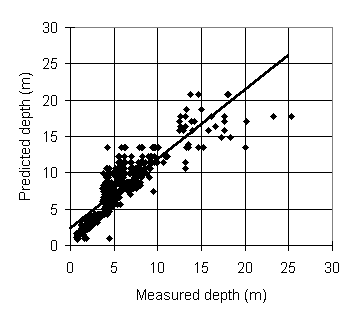
Using the ground measurements of depth listed in the spreadsheet DEPTHS.XLS one can compare the depths predicted by the image at each UTM coordinate with those measured on site using a depth sounder. The results of plotting measured depth against predicted depth for the image made using the modified Jupp's method are presented in Figure 4.3.
This method produced a correlation of 0.82 between predicted and measured depth but required extensive field bathymetric data. Even this method does not produce bathymetric maps suitable for navigation since the average difference between depths predicted from imagery and ground-truthed depths ranged from about 0.8 m in shallow water (<2.5 m deep) to about 2.8 m in deeper water (2.5-20 m deep).
Clearly, although bathymetric maps which look quite nice can be made from optical satellite imagery they provide little more than crude maps of depth which may be quite useful in planning surveys but cannot be used for much more.
However, if you have understood this exercise in trying to predict depth from satellite imagery you will find it much easier to understand the next lesson which is all about trying to compensate for the effect of depth on bottom reflectance so that one can map submerged habitats.
References
Bullard, R.K., 1983, Detection of marine contours from Landsat film and tape. In Remote Sensing Applications in Marine Science and Technology, edited by A.P. Cracknell (Dordrecht: D.Reidel) pp. 373-381.
Jerlov, N.G., 1976, Marine Optics. (Amsterdam: Elsevier)
Jupp, D.L.B., 1988, Background and extensions to depth of penetration (DOP) mapping in shallow coastal waters. Proceedings of the Symposium on Remote Sensing of the Coastal Zone, Gold Coast, Queensland, September 1988, IV.2.1-IV.2.19.
Jupp, D.L.B., Mayo, K.K., Kuchler, D.A., Classen, D van R., Kenchington, R.A. and Guerin., P.R., 1985, Remote sensing for planning and managing the Great Barrier Reef Australia. Photogrammetrica 40: 21-42.
Lyzenga, D.R., 1978, Passive remote sensing techniques for mapping water depth and bottom features. Applied Optics 17: 379-383.
Lyzenga, D.R., 1981, Remote sensing of bottom reflectance and water attenuation parameters in shallow water using aircraft and Landsat data. International Journal of Remote Sensing 2: 71-82.
Lyzenga, D.R., 1985, Shallow water bathymetry using a combination of LIDAR and passive multispectral scanner data. International Journal of Remote Sensing 6: 115-125.
Lantieri, D., 1988, Use of high resolution satellite data for agricultural and marine applications in the Maldives. Pilot study on Laamu Atoll. Fisheries and Agricultural Organisation Technical Report TCP/MDV/4905. No. 45.
Pirazzoli, P.A., 1985, Bathymetry mapping of coral reefs and atolls from satellite. Proceedings of the 5th International Coral Reef Congress, Tahiti, 6: 539-545.
Warne, D.K., 1978, Landsat as an aid in the preparation of hydrographic charts. Photogrammetric Engineering and Remote Sensing 44 (8): 1011-1016.
Van Hengel, W. and Spitzer, D., 1991, Multi-temporal water depth mapping by means of Landsat TM. International Journal of Remote Sensing 12: 703-712.
Zainal, A.J.M., Dalby, D.H., and I.S. Robinson., 1993,
Monitoring marine ecological changes on the east coast of Bahrain with
Landsat TM. Photogrammetric Engineering and Remote Sensing 59
(3): 415-421.
|
|
||||
|
|
|
|
|
|
| Maximum deepwater DN value (L deep max) |
|
|
|
|
| Minimum deepwater DN value (L deep min) |
|
|
|
|
| Mean/modal deepwater DN value (L deep mean) |
|
|
|
|
Depth range of boundary pixels: 18.70-25.35 m
|
|
|
|||
|
20.14
|
62
|
|||
|
25.35
|
61
|
|||
|
23.20
|
61
|
|||
|
21.01
|
60
|
|
||
|
20.45
|
59
|
|
|
|
|
> V deep max
|
20.09
|
59
|
21.7
|
20.8
|
|
<= V deep max
|
21.04
|
57
|
19.9
|
|
|
20.09
|
57
|
|||
|
18.70
|
56
|
Table 4.3. Calculating the maximum depth of penetration (zi).
|
|
||||
|
|
|
|
|
|
| Depth of deepest pixel with DN > L deep max |
|
|
|
|
| Depth of shallowest pixel with DN <= L deep max |
|
|
|
|
| Average depth of boundary pixels with DN values > L deep max |
|
|
|
|
| Average depth of boundary pixels with DN values = L deep max |
|
|
|
|
| Estimated maximum depth of penetration (zi) |
|
|
|
|
Estimating the depth of penetration (z2) for TM band 2.
Depth range of boundary pixels: 12.46-15.26 m
|
|
|
|||
|
13.14
|
20
|
|||
|
13.14
|
19
|
|||
|
15.26
|
17
|
|||
|
14.65
|
17
|
|
||
|
13.50
|
17
|
|
|
|
|
> V deep max
|
13.26
|
17
|
13.8
|
13.5
|
|
= V deep max
|
14.20
|
16
|
13.2
|
|
|
13.95
|
16
|
|||
|
13.85
|
16
|
|||
|
13.70
|
16
|
|||
|
13.50
|
16
|
|||
|
13.15
|
16
|
|||
|
13.15
|
16
|
|||
|
12.98
|
16
|
|||
|
12.77
|
16
|
|||
|
12.65
|
16
|
|||
|
12.54
|
16
|
|||
|
12.48
|
16
|
|||
|
12.46
|
16
|
| TM Band 1 | TM Band 2 | TM Band 3 | TM Band 4 | |
| DOP 1 |
|
|||
| DOP 2 |
|
|||
| DOP 3 |
|
|||
| DOP 4 |
|
|||
| ki |
|
|
|
|
| Ai |
|
|
|
|
 |
Back to main page | Back to Module 7 | USDOC | NOAA | NESDIS | CoastWatch |